Radial Basis Function Network and Support Vector Machine

1. Radial Basis Function Networkand Support Vector Machine Team 1: J-X Huang, J-H Kim, K-S Cho 2003. 10. 29

2. Outline • Radial Basis Function Network • Introduction • Architecture • Learning Strategies • MLP vs RBFN • Support Vector Machine • Introduction • VC Dimension, Structural Risk Minimization • Linear Support Vector Machine • Nonlinear Support Vector Machine • Conclusion

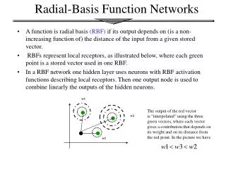
3. Radial Functions • Characteristic Feature • Response decreases (or increase) monotonically with distance from a central point.

4. Radial Basis Function Network • A kind of supervised neural networks, a feedforward network with three layers • Approximate function with linear combination of Radial basis functions F(x) = S wi G(||x-xi||) i = 1, 2, … , M • G(||x-xi||) is Radial Basis Function • Mostly Gaussian function • When M=number of sample, regularization network • When M<number of sample, we call it Radial-basis function network

5. 1 wo x1 x2 w1 ... ... wj ... Xp-1 wm Xp Output layer Hidden layer of Radial basis Functions Input layer Architecture

6. Three Layers • Input layer • Source nodes that connect to the network to its environment • Hidden layer • Each hidden unit (neuron) represents a single radial basis function • Has own center position and width (spread) • Output layer • Linear combination of hidden functions

7. Radial Basis Function m f(x) =  wjhj(x) j=1 hj(x)= exp( -(x-cj)2 / rj2 ) Where cj is center of a region, rj is width of the receptive field

8. Simple Summary on RBFN • A Feedforward Network • A linear model with a radial basis function • Three layers: • Input layer, hidden layer, output layer • Each hidden unit • Represents a single radial basis function • Has own center position and width (spread) • Parameter • Center, breath, weight

9. Example

10. Design • Require • Number of radial basis neurons • Selection of the center of each neuron • Selection of the each breath (width) parameter

11. Number of Radial Basis Neurons • Decide by designer • Max of neurons = number of input • Min of neurons will be experimentally determined • More neurons • More complex, but smaller tolerance • Spread: the selectivity of the neuron

12. Spread = 1/Selectivity

13. If Spread Too Small/Large

14. Learning Strategies • Two Levels of Learning • Center and spread learning (or determination) • Output layer weights learning • Fixed Center Selection • Self-organizing Center Selection • Supervised Selection of Centers with Weights • Make # (parameter) small as possible • Principles of dimensionality

15. Fixed Center Selection • Fixed RBFs of the hidden units • The locations of the centers may be chosen randomly from the training data set. • We can use different values of centers and widths for each radial basis function -> experimentation with training data is needed. • Only ouput layer weight is need to be learned • Obtain the value of the output layer weight by pseudo-inverse method • Main problem: require a large training set for a satisfactory level of performance

16. Self-Organized Selection of Center • Self-organized learning of centers by means of clustering • Clustering on the Hidden Layer • K-means clustering • Initialization • Sampling • Similarity matching • Updating • Continuation

17. Self-Organized Selection of Center (cont.) • Setting spreads • By selecting the average distance between center and the c closest points in the cluster (e.g. c=5) • Supervised learning on the output Layer • Estimate the connection weights w by the iterative gradient descent method based on least squares

18. Supervised Selection of Centers • All free parameters are changed by supervised learning process • The center is selected with the weight learning • Error-correction learning using least mean square (LMS) algorithm • Training for centers and spreads is very slow

19. Learning Formula • Linear weights (output layer) • Positions of centers (hidden layer) • Spreads of centers (hidden layer)

20. Approximation • RBF: Local network • Only inputs near a receptive field produce an activation • Can give “don’t know” output • MLP: Global network • All inputs cause an output

21. MLP vs RBFN

22. MLP vs. RBFN (cont)

23. In MLP

24. In RBFN

25. Outline • Radial Basis Function Network • Introduction • Radial Basis Function • Model • Training • Support Vector Machine • Introduction • VC Dimension, Structural Risk Minimization • Linear Support Vector Machine • Nonlinear Support Vector Machine • Conclusion

26. Introduction • Objective • Find an optimal hyperplane to: • Classify data points as much as possible • Separate the points of two classes as far as possible • Approach • Formulate a constrained optimization problem • Solve it using constrained quadratic programming (constrained QP) • Theorem • Structural Risk Minimization

27. Key Idea: Transform to Higher Dimensional Space

28. Maximum margin hyperplan optimal hyperplan hyperplan Find the Optimal Hyperplan

29. Maximize the Margin

30. Description on SVM • Given • A set of data points belong to either of two classes • SVM: Finds the Optimal Hyperplane • Minimizes the risk of misclassifying the training samples and unseen test samples • Maximizing the distance of either class from the hyperplane

31. Outline • Introduction • VC Dimension, Structural Risk Minimization • Linear Support Vector Machine • Nonlinear Support Vector Machine • Conclusion

32. Upper Bound for Expected Risk • Minimize the Expected Risk • Minimize the h: VC dimension • Minimize the empirical risk

33. True Risk Classification Error underfitting overfitting Confidence Interval Empirical Risk h(VC-dim.) VC Dimension and Empirical Risk • Empirical Risk is Decreasing Function of VC Dimension • Need a principled methods for the minimization

34. Structural Risk Minimization • Why Structural Risk Minimization (SRM) • It is not enough to minimize the empirical risk • Need to overcome the problem of choosing an appropriate VC dimension • SRM Principle • To minimize the expected risk, both sides in VC bound should be small • Minimize the empirical risk and VC confidence simultaneously • SRM picks a trade-off in between VC dimension and empirical risk

35. Outline • Introduction • VC Dimension, Structural Risk Minimization • Linear Support Vector Machine • Nonlinear Support Vector Machine • Performance and Application • Conclusion

36. Separable Case • Set S is Linearly Separable, then • The same as

37. Canonical Optimal Hyperplane w: normal to the hyperplan; is inverse proportion to the perpendicular distance from the hyperplane to the origin

38. Optimal Condition

39. Optimal Margin Hyperplane: Example

40. Non-Separable Case

41. Soft Margin Hyperplane

42. Kernels • Idea • Use a transformation (x) from input space to higher dimensional space • Find the separating hyperplane, make the inverse transformation • Kernel: dot product in a Banach space • Mercer’s Condition

43. Kernels for Nonlinear SVMs: Example • Polynomial Kernels • Neural Network Like Kernel • Radial Function Kernel

44. Kernel Example

45. Conclusion • Advantages • Efficient training algorithm (vs. multi-layer NN) • Represent complex and nonlinear functions (vs. single-layer NN) • Always find a global minimum • Disadvantages • Solution usually cubic in the number of training data • Large training set is a problem

46. Backup Slides

47. Radial Basis Function Network

48. Introduction • Radial Basis Function Network • A class of single hidden layer feedforward networks • Activation functions for hidden units are defined as radially symmetric basis functions such as the Gaussian function. • Advantages over Multi-Layer perceptron • Faster convergence • Smaller extrapolation errors • Higher reliability

49. Two Typical Radial Functions • Multi quaric RBF and Gaussian RBF

50. Modeling