Segmentation
Segmentation. . Segmentation : the problem. Identifying entities in the image, e.g. objects :. grouping pixels into segments crucial and basically unsolved step. . Segmentation : importance. Understanding scenes Industrial inspection Disease diagnosis …. .

Segmentation
E N D
Presentation Transcript
Segmentation : the problem Identifying entities in the image, e.g. objects : • grouping pixels into segments • crucial and basically unsolved step
Segmentation : importance • Understanding scenes • Industrial inspection • Disease diagnosis • ….
Learning objectives: What can you do after today • Describe image segmentation task • Implement thresholding based techniques: • Morphological operators • Separating multiple components with region growing • Describe their limitations • Implement Hough transform to find lines, describe advantages and limitations • Describe different statistical pattern recognition based methods • Clustering • Supervised generative models • Discriminative learning principles
Segmentation : Outline • Thresholding • Edge based • Region based • Statistical Pattern Recognition based
Segmentation : Outline • Thresholding • Edge based • Region based • Statistical Pattern Recognition based
Thresholding : principle For high contrasts between objects and background Determine intensity threshold that defines 2 pixel categories : object and background Example image :
Thresholding : basic idea Histogram Threshold = 5 Threshold = 25 Threshold = 50 Threshold = 70
Thresholding : threshold selection Histogram Alternatives: If intensities are known - easy Take the minimum between two peaks Reach a predefined area – for industrial application Maximize sum of gradients at pixels with threshold intensity Low gradient magnitude areas Use regions with high response to Laplacian filter – points around the edge
Thresholding: Otsu criterion[Nobuyuki Otsu] Minimize within-group variance Group 1 I > threshold Group 2 I <= threshold Otsu threshold = 35
Fixed threshold Image specific Otsu threshold Local Otsu threshold Thresholding: Otsu versus fixed
What happens with noise? An example :
What happens with noise? Pixels can fall on the wrong side of the threshold Threshold at 35:
Solution: Enhancement of binary images Remove the isolated islands in the binary images Mathematical morphology
Basics of Mathematical Morphology • Operations on binary images • Shift-invariant • Non-linear • Based on neighboring pixelsdefined through structural elements • View binary images as sets • Two main operations Binary Image: A Dilation Erosion Binary structural element: B
On the noisy segmentation Erosion Dilation
Concatenation of basic operations: Opening and closing Opening Closing
Opening and closing Opening Closing
Binary enhancement as rank order operators New intensity based on rank-ordered neighborhood values – Extension to gray level images Important difference with convolution : non-linearity
Binary enhancement : remarks • 1. Post-processing approach Many alternatives to enforce neighborhood consistency during segmentation • 2. Erosion + dilation (opening) Dilation + erosion (closing) • 3. Noise in background can be reduced by reversed operation • 4. Use same neighbourhood for both steps • 5. Reminder : median filtering useful for edge preserving smooting
Multiple objects: Connected components We would like to separate these objects Connected component analysis What does it mean to be a connected object?
The structure of discrete image spaces Two main aspects • Topology • Distance Strong relationship
Topology • The problem of the bridges of KönigsbergPrusia (Today’s Russia - Kaliningrad) • Solution: Euler, 1736 • The birth of graph theory • Independent of distances
Formal definition • Topological space • is a set of points, • are the open subsets above • Describes the neighbourhood structure of a space
Neighbourhood of the Cartesian image raster • Defined by the pixel neighbourhood structure • There is no unique definition • 4- and 8-connectivity the most popular • There are other possibilities
Topology of discrete binary images • Defined by connectivity (Neighbourhood C ) • Connected pixels through neighbourhood chain such that and • Two components: Foreground, Background • Connected component: if every two point are connected through the same component • Topology defined by the number of FG/BG components
Determination of topology • Region growing • Components can be found one by one until all are labeled
Connected component labeling • Scanning the image line-by-line (TV scan) enforces an (artificial) causality • At every pixel the neighbourhood divided into past and future • All labels on past pixels collected. Possible options • No label found: give a new label • One label found: propagate it to the central pixel • More than one label found: note their equivalence • At the end equivalent components (connected but labelled as different) have to be re-labeled
Distance on the image raster • is a metrics over if • One can define open and closed disks with center P and radius r which can be used to define neighbourhoods • Intimate connection between topology and metrics
Topology induced metrics • Defined based on connectivity • Length of connecting paths (number of steps) • Minimal length between all connecting paths • D4(Manhattan) and D8 distances e.g. • How to calculate between P(i,j) and Q(k,l)? • Circles in D4 and D8? • Euclidean not conform with any discrete neighbourhood
Distance calculation • Distance transformations: distance maps based on distance propagation along neighbourhoods • Euclidean distance map • True implementation is very cumbersome • Approximation by increasingly large neighbourhoods
Thresholding : remarks • Threshold advantages: 1. Serious bandwidth reduction 2. Simplification of further processing 3. Availability of real-time hardware for shape recognition • Generally it won’t provide a satisfying segmentation • Sometimes several thresholds yields finer labelling usually infeasible • Pixel-by-pixel decision • ignores neighbouring pixels • structural information lost
bone liver blood tumour kidney heart pancreas intestine water breast fat lung air Thresholding has limitations X-ray attenuation is tissue dependent • strong overlap • limited separability on histogram
Segmentation : Outline • Thresholding • Edgebased • Region based • Statistical Pattern Recognition based
Thresholding is not enough: Edges can help Identifying boundaries between different segments / objects Image After thresholding with Otsu criteria Edge Detection with Canny
Edge linking techniques • 1. Hough Transform: for predefined shapes • 2. Elastically deformable contour models Snakes: generic shape priors [Next week] • 3. Many other methods for grouping combination with user interaction (dynamic path search – in the script)
The Hough transform : principle Uses parametric shape models to extract objects in lower dimensional spaces In other words, if you know the shape, then Hough Transform can be used to detect it. The simplest example: straight lines Many further possibilities, like circles, ellipses andgeneralizations to other shapes
e.g. straight edges in object outlines in all possible positions and orientations. Hough transform : straight lines Suppose we would like to detect straight lines for general shapes : 3 degrees of freedom Allowing three-dimensional rotations the situation would even get more complex Straight lines, however, will remain invariant under several such transformations The image projection of a straight line is fully characterized by 2 parameters
The Hough transform : • 1. Inspect all points of interest • 2. For each point draw the above line in (a,b) - parameter space Hough transform : straight lines We write the equation of a straight line as Fixing a point (x,y), all lines through the point :
Hough transform : straight lines implementation : 1. the parameter space is discretised 2. a counter is incremented at each cell where the lines pass 3. peaks are detected
Hough transform : straight lines problem : unbounded parameter domain vertical lines require infinite a alternative representation: Each point will add a sinusoidal function in the (ρ,𝜽) parameter space
Hough transform : straight lines Square : Circle :
Hough transform : straight lines combined:
Hough transform : remarks • 1. time consuming • 2. robust, to noise, … • 3. peak detection is difficult • 4. Robustness of peak detection increased by weighting contributions (e.g in examples weighting with intensity gradient magnitude) • 5. Ambiguities possible – if similar objects are close by…
Segmentation : Outline • Thresholding • Edge based • Region based • Statistical Pattern Recognition based