Download
1 / 33
380 likes | 795 Vues
Learn the basic laws of vector algebra, orthogonal coordinate systems, transformations, and operations like divergence, curl, gradient, and Laplacian in this chapter. Understand vector products and applications in electromagnetics.

E N D
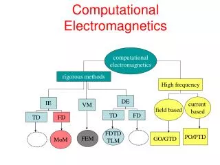
Fundamentals of Applied Electromagnetics Chapter 2 - Vector Analysis
Chapter Objectives • Operations of vector algebra • Dot product of two vectors • Differential functions in vector calculus • Divergence of a vector field • Divergence theorem • The curl of a vector field • Stokes’s theorem
Chapter Outline 2-1) Basic Laws of Vector Algebra Orthogonal Coordinate Systems Transformations between Coordinate Systems Gradient of a Scalar Field Divergence of a Vector Field Curl of a Vector Field Laplacian Operator 2-2) 2-3) 2-4) 2-5) 2-6) 2-7)
2-1 Basic Laws of Vector Algebra • Vector A has magnitudeA = |A| to the direction of propagation. • Vector A is shown and represented as
2-1.1 Equality of Two Vectors • A and B are equal when they have equal magnitudes and identical unit vectors. • For addition and subtraction of A and B, 2-1.2 Vector Addition and Subtraction
2-1.3 Position and Distance Vectors • Position vectoris the vector from the origin to point.
2-1.4 Vector Multiplication • 3 different types of product in vector calculus: • Simple Product with a scalar • Scalar or Dot Product where θAB= angle between A and B +ve -ve
2-1.4 Vector Multiplication 3. Vector or Cross Product • Cartesian coordinate system relations: • In summary,
2-1.5 Scalar and Vector Triple Products • A scalar triple product is • A vector triple product is known as the “bac-cab” rule.
Example 2.2 Vector Triple Product Given , , and , find (A× B)× C and compare it with A× (B× C). Similar procedure will give Solution
2-2 Orthogonal Coordinate Systems • Orthogonal coordinate systemhas coordinates that are mutually perpendicular. • Differential length in Cartesian coordinates is a vector defined as 2-2.1 Cartesian Coordinates
2-2.2 Cylindrical Coordinates • Base unit vectors obey right-hand cyclic relations. • Differential areas and volume in cylindrical coordinatesare shown.
Example 2.4 Cylindrical Area Find the area of a cylindrical surface described by r = 5, 30° ≤ Ф ≤ 60°, and 0 ≤ z ≤ 3 For a surface element with constant r,the surface area is Solution
2-2.3 Spherical Coordinates • Base unit vectors obey right-hand cyclic relations. where R = rangecoordinate sphere radius Θ = measured from the positive z-axis
Example 2.6 Charge in a Sphere A sphere of radius 2 cm contains a volume charge density ρv given by Find the total charge Q contained in the sphere. Solution
2-3 Transformations between Coordinate Systems Cartesian to Cylindrical Transformations • Relationships between (x, y, z) and (r, φ, z) are shown. • Relevant vectors are defined as
2-3 Transformations between Coordinate Systems Cartesian to Spherical Transformations • Relationships between (x, y, z) and (r, θ, Φ) are shown. • Relevant vectors are defined as
Example 2.8 Cartesian to Spherical Transformation Express vector in spherical coordinates. Using the transformation relation, Using the expressions for x, y, and z, Solution
Solution 2.8 Cartesian to Spherical Transformation Similarly, Following the procedure, we have Hence,
2-3 Transformations between Coordinate Systems Distance between Two Points • Distance d between 2 points is • Converting to cylindrical equivalents. • Converting to spherical equivalents.
2-4 Gradient of a Scalar Field • Differential distance vector dl is . • Vector that change position dl is gradient of T, or grad. • The symbol is called the del or gradient operator.
2-4 Gradient of a Scalar Field • Gradient operator needs to be scalar quantity. • Directional derivativeof Tis given by • Gradient operator in cylindrical and spherical coordinates is defined as 2-4.1 Gradient Operator in Cylindrical and Spherical Coordinates
Example 2.9 Directional Derivative Find the directional derivative of along the direction and evaluate it at (1,−1, 2). Gradient of T : We denote l as the given direction, Unit vector is and Solution
2-5 Divergence of a Vector Field • Total flux of the electric field E due to q is • Flux lines of a vector field E is
2-5.1 Divergence Theorem • The divergence theorem is defined as • ∇ ·E stands for the divergence of vector E.
Example 2.11 Calculating the Divergence Determine the divergence of each of the following vector fields and then evaluate it at the indicated point: Solution
2-6 Curl of a Vector Field • Circulation is zero for uniform field and non-zero for azimuthal field. • The curl of a vector field B is defined as
2-6.1 Vector Identities Involving the Curl • Vector identities: (1) ∇ × (A + B) = ∇× A+∇× B, (2) ∇ ·(∇ × A) = 0 for any vector A, (3) ∇ × (∇V ) = 0 for any scalar function V. • Stokes’s theoremconverts surface into line integral. 2-6.2 Stokes’s Theorem
Example 2.12 Verification of Stokes’s Theorem A vector field is given by . Verify Stokes’s theorem for a segment of a cylindrical surface defined by r = 2, π/3 ≤ φ≤ π/2, and 0 ≤ z ≤ 3, as shown. Solution Stokes’s theorem states that Left-hand side: Express in cylindrical coordinates
Solution 2.12 Verification of Stokes’s Theorem The integral of ∇ × B over the specified surface S with r = 2is Right-hand side: Definition of field B on segments ab, bc, cd, and da is
Solution 2.12 Verification of Stokes’s Theorem At different segments, Thus, which is the same as the left hand side (proved!)
2-7 Laplacian Operator • Laplacianof V is denoted by ∇2V. • For vector E given in Cartesian coordinates as the Laplacian of E is defined as
2-7 Laplacian Operator • In Cartesian coordinates, the Laplacian of a vector is a vector whose components are equal to the Laplacians of the vector components. • Through direct substitution, we can simplify it as