Download
1 / 21
210 likes | 232 Vues
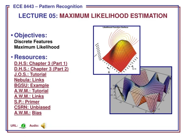
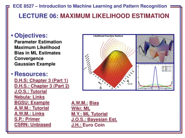
This slideshow discusses the concept of maximum-likelihood estimation (MLE) in pattern classification, using examples from the Gaussian case. It covers topics such as estimating parameters, bias in MLE, and the problem statement for MLE.

E N D
Pattern ClassificationAll materials in these slides were taken fromPattern Classification (2nd ed) by R. O. Duda, P. E. Hart and D. G. Stork, John Wiley & Sons, 2000 with the permission of the authors and the publisher
Introduction Maximum-Likelihood Estimation Example of a Specific Case The Gaussian Case: unknown and Bias Appendix: ML Problem Statement Chapter 3:Maximum-Likelihood & Bayesian Parameter Estimation (part 1)
Introduction • Data availability in a Bayesian framework • We could design an optimal classifier if we knew: • P(i) (priors) • P(x | i) (class-conditional densities) Unfortunately, we rarely have this complete information! • Design a classifier from a training sample • No problem with prior estimation • Samples are often too small for class-conditional estimation (large dimension of feature space!) Pattern Classification, Chapter 3 1
A priori information about the problem • Do we know something about the distribution? • find parameters to characterize the distribution • Example: Normality of P(x | i) P(x | i) ~ N( i, i) • Characterized by 2 parameters • Estimation techniques • Maximum-Likelihood (ML) and the Bayesian estimations • Results are nearly identical, but the approaches are different Pattern Classification, Chapter 3 1
Parameters in ML estimation are fixed but unknown! • Best parameters are obtained by maximizing the probability of obtaining the samples observed • Bayesian methods view the parameters as random variables having some known distribution • In either approach, we use P(i | x)for our classification rule! Pattern Classification, Chapter 3 1
Maximum-Likelihood Estimation • Has good convergence properties as the sample size increases • Simpler than any other alternative techniques • General principle • Assume we have c classes and P(x | j) ~ N( j, j) P(x | j) P (x | j, j) where: Pattern Classification, Chapter 3 2
Use the informationprovided by the training samples to estimate = (1, 2, …, c), each i (i = 1, 2, …, c) is associated with each category • Suppose that D contains n samples, x1, x2,…, xn • ML estimate of is, by definition the value that maximizes P(D | ) “It is the value of that best agrees with the actually observed training sample” Pattern Classification, Chapter 3 2
Optimal estimation • Let = (1, 2, …, p)t and let be the gradient operator • We define l() as the log-likelihood function l() = ln P(D | ) (recall D is the training data) • New problem statement: determine that maximizes the log-likelihood Pattern Classification, Chapter 3 2
The definition of l() is: and Set of necessary conditions for an optimum is: l = 0 (eq. 7) Pattern Classification, Chapter 3 2
Example, the Gaussian case: unknown • We assume we know the covariance • p(xi | ) ~ N(, ) (Samples are drawn from a multivariate normal population) = therefore:The ML estimate for must satisfy: Pattern Classification, Chapter 3 2
Multiplying by and rearranging, we obtain: Just the arithmetic average of the samples of the training samples! Conclusion: If P(xk | j) (j = 1, 2, …, c) is supposed to be Gaussian in a d-dimensional feature space; then we can estimate the vector = (1, 2, …, c)t and perform an optimal classification! Pattern Classification, Chapter 3 2
Example, Gaussian Case: unknown and S • First consider univariate case: unknown and = (1, 2) = (, 2) Pattern Classification, Chapter 3 2
Summation (over the training set): Combining (1) and (2), one obtains: Pattern Classification, Chapter 3 2
The ML estimates for the multivariate case is similar • The scalars c and are replaced with vectors • The variance s2 is replaced by the covariance matrix Pattern Classification, Chapter 3
Bias • ML estimate for 2 is biased • Extreme case: n=1, E[ ] = 0 ≠ 2 • As the n increases the bias is reduced this type of estimator is called asymptotically unbiased Pattern Classification, Chapter 3 2
An elementary unbiased estimator for is: This estimator is unbiased for all distributions Such estimators are called absolutely unbiased Pattern Classification, Chapter 3 2
Our earlier estimator for is biased: In fact it is asymptotically unbiased: Observe that Pattern Classification, Chapter 3 2
Appendix: ML Problem Statement • Let D = {x1, x2, …, xn} P(x1,…, xn | ) = 1,nP(xk | ); |D| = n Our goal is to determine (value of that maximizes the likelihood of this sample set!) Pattern Classification, Chapter 3 2
|D| = n . . . . x2 . . x1 xn N(j, j) = P(xj, 1) P(xj | 1) P(xj | k) D1 x11 . . . . x10 Dk . Dc x8 . . . x20 . . x1 x9 . . Pattern Classification, Chapter 3 2
= (1, 2, …, c) Problem: find such that: Pattern Classification, Chapter 3 2