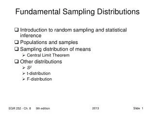
Chapter 8: Fundamental Sampling Distributions and Data Descriptions: 8.1 Random Sampling:
220 likes | 321 Vues
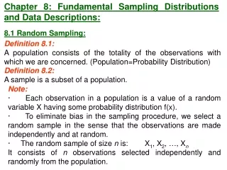
Chapter 8: Fundamental Sampling Distributions and Data Descriptions: 8.1 Random Sampling:. Definition 8.1: A population consists of the totality of the observations with which we are concerned. (Population=Probability Distribution). Definition 8.2: A sample is a subset of a population. Note:

Chapter 8: Fundamental Sampling Distributions and Data Descriptions: 8.1 Random Sampling:
E N D
Presentation Transcript
Chapter 8: Fundamental Sampling Distributions and Data Descriptions: 8.1 Random Sampling: Definition 8.1: A population consists of the totality of the observations with which we are concerned. (Population=Probability Distribution) Definition 8.2: A sample is a subset of a population. Note: · Each observation in a population is a value of a random variable X having some probability distribution f(x). · To eliminate bias in the sampling procedure, we select a random sample in the sense that the observations are made independently and at random. · The random sample of size n is: X1, X2, …, Xn It consists of n observations selected independently and randomly from the population.
Central Tendency in the Sample: Definition 8.5: If X1, X2, …, Xn represents a random sample of size n, then the sample mean is defined to be the statistic: (unit) Note: · is a statistic because it is a function of the random sample X1, X2, …, Xn. · has same unit of X1, X2, …, Xn. · measures the central tendency in the sample (location). 8.2 Some Important Statistics: Definition 8.4: Any function of the random sample X1, X2, …, Xn is called a statistic.
Variability in the Sample: Definition 8.9: If X1, X2, …, Xn represents a random sample of size n, then the sample variance is defined to be the statistic: (unit)2 Theorem 8.1: (Computational Formulas for S2) Note: · S2 is a statistic because it is a function of the random sample X1, X2, …, Xn. · S2 measures the variability in the sample. (unit)
8.4 Sampling distribution: Definition 8.13: The probability distribution of a statistic is called a sampling distribution. · Example: If X1, X2, …, Xn represents a random sample of size n, then the probability distribution of is called the sampling distribution of the sample mean . 8.5 Sampling Distributions of Means: Result: If X1, X2, …, Xn is a random sample of size n taken from a normal distribution with mean and variance 2, i.e. N(,), then the sample mean has a normal distribution with mean Example 8.1: Reading Assignment Example 8.8: Reading Assignment Example 8.9: Reading Assignment
and variance · If X1, X2, …, Xn is a random sample of size n from N(,), then ~N( , ) or ~N(, ).
Theorem 8.2: (Central Limit Theorem) If X1, X2, …, Xn is a random sample of size n from any distribution (population) with mean and finite variance 2, then, if the sample size n is large, the random variable is approximately standard normal random variable, i.e., approximately. • We consider n large when n30. • For large sample size n, has approximately a normal distribution with mean and variance , i.e., approximately.
The sampling distribution of is used for inferences about the population mean . Solution: X= the length of life =800 , =40 X~N(800, 40) n=16 Example 8.13: An electric firm manufactures light bulbs that have a length of life that is approximately normally distributed with mean equal to 800 hours and a standard deviation of 40 hours. Find the probability that a random sample of 16 bulbs will have an average life of less than 775 hours.
Sampling Distribution of the Difference between Two Means: Suppose that we have two populations: · 1-st population with mean 1 and variance 12 · 2-nd population with mean 2 and variance 22 · We are interested in comparing 1 and 2, or equivalently, making inferences about 12. · We independently select a random sample of size n1 from the 1-st population and another random sample of size n2 from the 2-nd population: · Let be the sample mean of the 1-st sample. · Let be the sample mean of the 2-nd sample. · The sampling distribution of is used to make inferences about 12.
Theorem 8.3: If n1 and n2 are large, then the sampling distribution of is approximately normal with mean and variance that is: Note:
Example 8.15: Reading Assignment Example 8.16: The television picture tubes of manufacturer A have a mean lifetime of 6.5 years and standard deviation of 0.9 year, while those of manufacturer B have a mean lifetime of 6 years and standard deviation of 0.8 year. What is the probability that a random sample of 36 tubes from manufacturer A will have a mean lifetime that is at least 1 year more than the mean lifetime of a random sample of 49 tubes from manufacturer B? Solution: Population A Population B 1=6.5 2=6.0 1=0.9 2=0.8 n1=36 n2=49
· We need to find the probability that the mean lifetime of manufacturer A is at least 1 year more than the mean lifetime of manufacturer B which is P( ). · The sampling distribution of is
Recall = P(Z2.65) = 1 P(Z<2.65)= 1 0.9960 = 0.0040
8.7 t-Distribution: · Recall that, if X1, X2, …, Xn is a random sample of size n from a normal distribution with mean and variance 2, i.e. N(,), then · We can apply this result only when 2 is known! If 2 is unknown, we replace the population variance 2 with the sample variance · to have the following statistic
Result: If X1, X2, …, Xn is a random sample of size n from a normal distribution with mean and variance 2, i.e. N(,), then the statistic has a t-distribution with =n1degrees of freedom (df), and we write T~ t(). • Note: • t-distribution is a continuous distribution. • The shape of t-distribution is similar to the shape of the standard normal distribution.
Notation: • t= The t-value above which we find an area equal to , that is P(T> t) = • Since the curve of the pdf of T~ t() is symmetric about 0, we have • t1 = t • Values of t are tabulated in Table A-4 (p.683).
Example: Find the t-value with =14 (df) that leaves an area of: (a) 0.95 to the left. (b) 0.95 to the right. Solution: = 14 (df); T~ t(14) (a) The t-value that leaves an area of 0.95 to the left is t0.05 = 1.761
(b) The t-value that leaves an area of 0.95 to the right is t0.95 = t 1 0.95= t 0.05= 1.761
Example: For = 10 degrees of freedom (df), find t0.10 and t 0.85 . Solution: t0.10 = 1.372 t0.85 = t10.85 = t 0.15 = 1.093 (t 0.15 = 1.093)