Download
1 / 17
180 likes | 337 Vues
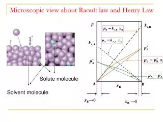
p. k x,B. k x,A. Solute molecule. Solvent molecule. A. B. x B. x B →0. x B →1. Microscopic view about Raoult law and Henry Law. Gas A,B y A ,y B. Liquid A, B x A ,X B. Ideal solution. The solvent and solute both follow Raoult Law. Binary system. Scuba diving.

E N D
p kx,B kx,A Solute molecule Solvent molecule A B xB xB→0 xB→1 Microscopic view about Raoult law and Henry Law
Gas A,B yA,yB Liquid A, B xA,XB Ideal solution The solvent and solute both follow Raoult Law Binary system
Scuba diving Vaporizable solutes follow Henry Law 25℃, sea level, O2 in air PO2=21kPa
kA P xA Chemical potential of B, X=1, follow Henry Law Ideal diluted solution Solvent follow Raoult’s law Solute follow Henry’s law
Chemical potential of reference/standard state: Solute in diluted solution
solute solvent 4.5 Colligative properties of diluted solution The solute is not volatile The decrease of vaporizing pressure Freezing-point depression The elevation of boiling point Osmosis: osmotic pressure
Freezing-point depression (l) (s) Tf* (sln) (s) Tf 1(sln) = 1*(s) 1y(l) + RT ln x1 = 1y(s) RT ln x1 = –[1y(l) – 1y(s) ]
X2 is small lnx1=ln(1– x2) x2 Tf should be small, too freezing point lowering coefficients Note: diluted solution, separate pure solid (solvent)
Boiling-point elevation (boiling point elevation coefficients),Unit:
Semipermeable membrane Osmosis pressure Osmosis phenomenon and osmosis pressure A(sln)=Ay(l) + RT ln xA<A*(l) P↑, μ ↑
Osmosis pressure: meaning, measurement and application Van’t Hoff equation Δp=0.053Pa;ΔTf=0.002K; π=2400Pa 20℃,mB=0.001mol.kg-1
Colligative properties of diluted solution: Application examples • Mr. Tian Wen-fei • Mr. Tian Wen-zhi
γcs2 γacetone 4.6 Real solution: activity of solute and solvent By R.L. Judged by Raoult law Or by Henry Law
Determination of activity of solvent (1) p1 = p1* a1
Example 1: Activity of water in aqueous solution P0, Aqueous solution Tf=– 15℃ Question: a(water)=? Osmosis pressure of the solution. Answer: a1=0.857
40000Pa P PB PA 1 0 xA Example 2: Acetic acid(A)/benzene(B) solution By R.L: By R.L By H.L mixG=RT(xA ln aA + xB ln aB)= – 1167J
Homeworks • Y:P101:15; P104:17,18 P106: 22 • P110:23 • A: P190: Exe7.19(b); Problem7.1 • P192: application7.23 Term seminar report : May 21: May 23: May 30: June 04: June 06: 10 min/person