Estimating P(sentence) or P(document)

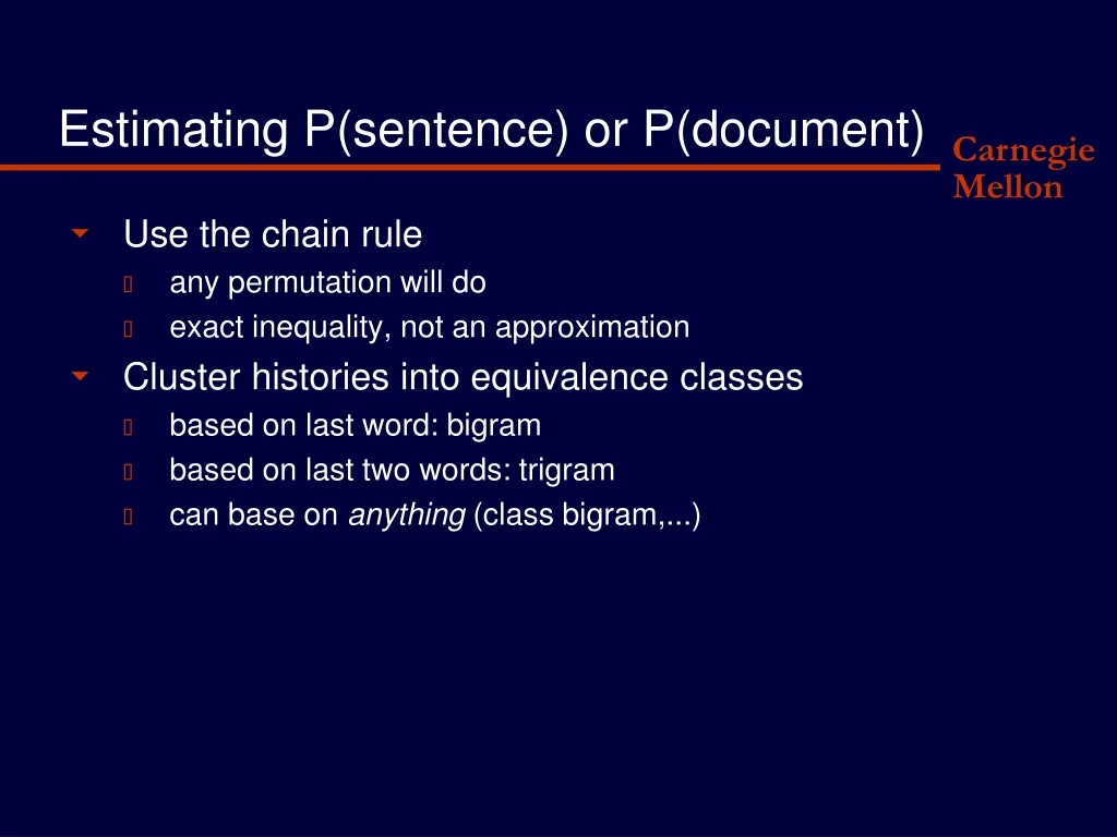
1. Estimating P(sentence) or P(document) • Use the chain rule • any permutation will do • exact inequality, not an approximation • Cluster histories into equivalence classes • based on last word: bigram • based on last two words: trigram • can base on anything (class bigram,...)

2. Interpolation Ngram • Create models of different orders: • zerogram (uniform), unigram, bigram, trigram... • each model can (but need not!) be smoothed • as model order increases • bias decreases (closer to P(w|h)) • variance increases (less data / more parameters) • Linearly interpolate all models • a form of shrinkage

3. Linearly interpolating multiple LMs • Not limited to Ngrams • any model can be interpolated (even a black box) • How to choose the interpolation weights? • maximize likelihood of new, unseen (aka heldout) data • this is not standard ML estimation of (models, weights) • it is ML estimation of the weights, given fixed models • good news: the likelihood function is convex in the weights • there is a single, global maximum • easy to find in a variety of methods • we use a simple variant of EM

4. Linear Interpolation (cont.) • Extremely general • Guaranteed not to hurt (provided heldout set is large enough to be representative) • “When in trouble, interpolate!” • Order of interpolation doesn’t matter • To determine optimal weights, actual LMs not needed, only their values (probability stream) on a common heldout set.

5. Economizing on Data • For the method described above, we need to pre-divide our data into training+heldout • Improvement #1: • divide data into two halves, A & B. • train components on A, estimate weights on B • train components on B, estimate weights on A • train components on A+B, use average weights from above • Problem: weights are optimal for half the data • with more data, optimal weights are likely different

6. Economizing on Data (cont.) • Improvement #2 (“block deleted interpolation”) • divide data into k (say, 10) equal-size parts • train on k-1 parts, estimate weights on remaining part • repeat k times, cycling thru all parts • train on entire set, use average weights from above • weights are now (nearly) optimal

7. Economizing on Data (cont.) • Improvement #3 (“leave-one-out”) • same as block-deleted-interpolation, but k=N (each block consists of a single data item) • must train N different models! • only feasible if models can be easily derived from each other by small modification

8. Linear Interpolation: Improvements • Weights can depend on the history h • Typically, histories will be clustered by their counts in the training data • large counts: larger weight to hi-var model (e.g. trigram) • small counts: larger weight to low-var model (e.g. unigram) • The “Brick” method (IBM): • cluster training histories acc. to C(Wi-2,Wi-1) and C(W i-1) • further cluster histories by “bricks” in this 2D space

9. The Backoff Model • Order models by increasing bias • If not enough evidence to use model K (variance too high), backoff to model K+1 (recursively) • Discount low-count events; discount mass distributed to lower-order model • Proposed by Katz in 1986, in conjunction with G-T discounting (but any discounting can be used!) • Simple to implement, surprisingly powerful • Corresponds to “non-linear shrinkage”, which became popular in statistics in the 2000’s.

10. Combining interpolation and Discounting • Discounting small events is sound and reduces the bias of the model • Historically it was only done with backoff models, but there’s no reason it can’t be used with the components of linear interpolation • This was tried for the first time in teh mid 90’s, with further improvement!