Download

1 / 26
260 likes | 459 Vues
Heat Conduction of Zinc Specimen. Femlab Simulation Measurement Calibration Technique: Effects of Heat Loss Through Specimen Surface Area . Experiment Objectives.

E N D
Heat Conduction of Zinc Specimen Femlab Simulation Measurement Calibration Technique: Effects of Heat Loss Through Specimen Surface Area
Experiment Objectives • The main objective in this experiment is to measure the effective thermal conductivities of a material within a temperature range of 77K-350K. • This will allow us to classify and identify any similarities discovered by the experimental data compared with published data on the specific material. • To familiarize ourselves with the concepts and principles that govern similar thermodynamic systems. • To gain insight and knowledge of various measurement techniques associated with thermal transport. • Also to become familiar with setup and use of various pieces of equipment needed to perform the experiment.
Theory and Concepts (2) --------------------------------------- (Short-Hand Notation) (Conduction along x-direction) These expressions lead to the 2nd Order Time Dependant Heat Diffusion Differential Equation, which has the following form: (non-linear, 3-D general form) -----------------------(General Heat Diffusion Relation)
Experiment Overview • Heat source – Used a resistor with a voltage running through it. Causes heat dissipation in the form of power (i.e heat flux) • Measurement Device (Thermocouples) – Carefully placed 2 thermo-sensors (30mm apart) in order to record data for at least two different spatial locations. • LABVIEW – Easily Recorded Measurements using the DAQ Assistant Box • GNU Octave (Data Analysis)
Data Acquisition • LABVIEW Data Acquisition Software • Recorded Measurements using a virtual instrument based software. • Directly converts measurements into temperatures rather than direct voltages. • Shell Script, GNU Octave • Shell script for command execution and file manipulation • GNU Octave for data manipulation, plotting, and analysis
Visual Of V.I. Instrumentation Block Diagram
Visual Of V.I. Instrumentation Temperature Output Interface
Experiment CAD Model Shows a rough CAD Model of the measurement apparatus. Consists of Zinc cylinder, hot plate (inward heat flux), and wiring to the LABVIEW DAQ box for measurement recording.
Application of FEMLAB • Problem: • Recorded measurements do not account for loss of energy due to convective heat flux through surface of cylinder. • Solution: • FEMLAB simulation was performed to adjust measurements to include convective energy losses. The results were used to compute the thermal conductivity of the material.
Sensor 2 2 Sensor 1 FEMLAB GEOMETRY • Sensor 1 was placed at z = .6 in the FEMLAB model of the system. • Sensor 2 was placed at z = 1.2, which gives a total separation distance = .6. • This will allow us to compare the temperature differences between the two sensors for the two cases: • Thermally Insulated Surface • Heat Loss Effects Through Sides Actual to Model Scaling: 1 unit = 50mm
FEMLAB Simulation Parameters • Modules • 2D – Incompressible Navier Stokes • 2D – Heat Diffusion Equation (Energy Transfer) • Simulation Geometry • Cylinder encapsulated by a rectangle box representing system’s physical boundaries. (I) • 2D – Axial Symmetric rectangle (cylinder) that was used for the energy transfer equation with the velocity solution of part 1. (II)
FEMLAB RESULTS • Phase I – Velocity Solution
Phase I – Velocity Solution (cont) Cylinder Boundary Viscous Drag Vs. Arc Length
Phase I – Velocity Solution (cont) Cylinder Boundary Vorticity Profiles Vortex Strength Vs. Arc Length Vortex Strength Vs. X - Distance
Phase II – Temperature Solution (Thermally Insulated) ∆T = 1.034483 degrees
Phase II – Temperature Solution (Convective Heat Loss Effects) ∆T = .732588 degrees
Phase II – Temperature Solution (Convective Heat Loss Effects) Heat Flux Profile Vs. Z – Direction
Simulation Results • When accounting for the heat flux through the side surfaces of the cylinder, the temperature difference is decreased by the following ratio: • Π = .732588 / 1.034483 = 0.708168 Which yields a percent reduction from the thermally insulated case to heat losses of: • Ψ = 1 – Π = 29.183 %
Measurement Results • Room Temperature Results Temperature Vs Time (for each Thermocouple)
Room Temperature Results (cont) Temperature Difference Vs. Time (steady–state time)
Liquid Nitrogen Results ( ≈77 K ) Heat Source was turned off at kink at about 9500 sec
Liquid Nitrogen Results ( ≈77 K ) (cont) Temperature Difference Vs. Time (note: Drastic Drop when heat source was turned off ≈9500 sec
Non-Dimensional Temperature Profile • Non-Dimensional Profile of Thermo1. Notice the spike at about 9540 sec. This is when T1 = T2 for a split second as a consequence of turning the heat source off and instant cooling occurs. θ1=(T1–To)/(T1–T2) & θ2=(T2–To)/(T1–T2)
Thermal Conductivity • TO BE CONTINUED…