Unsteady State Heat Conduction
MODULE 5. Unsteady State Heat Conduction . UNSTEADY HEAT TRANSFER.


Unsteady State Heat Conduction
E N D
Presentation Transcript
MODULE 5 Unsteady State Heat Conduction
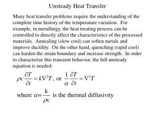
UNSTEADY HEAT TRANSFER Many heat transfer problems require the understanding of the complete time history of the temperature variation. For example, in metallurgy, the heat treating process can be controlled to directly affect the characteristics of the processed materials. Annealing (slow cool) can soften metals and improve ductility. On the other hand, quenching (rapid cool) can harden the strain boundary and increase strength. In order to characterize this transient behavior, the full unsteady equation is needed:
Fig. 5.1 “A heated/cooled body at Ti is suddenly exposed to fluid at T with a known heat transfer coefficient . Either evaluate the temperature at a given time, or find time for a given temperature.” Q: “How good an approximation would it be to say the annular cylinder is more or less isothermal?” A: “Depends on the relative importance of the thermal conductivity in the thermal circuit compared to the convective heat transfer coefficient”.
Biot No. Bi • Defined to describe the relative resistance in a thermal circuit of the convection compared Lc is a characteristic length of the body Bi→0: No conduction resistance at all. The body is isothermal. Small Bi: Conduction resistance is less important. The body may still be approximated as isothermal Lumped capacitance analysis can be performed. Large Bi: Conduction resistance is significant. The body cannot be treated as isothermal.
Solid Total Resistance= Rexternal + Rinternal GE: BC: Solution: Transient heat transfer with no internal resistance: Lumped Parameter Analysis Valid for Bi<0.1
Note: Temperature function only of time and not of space! Lumped Parameter Analysis • - To determine the temperature at a given time, or • To determine the time required for the • temperature to reach a specified value.
Thermal diffusivity:(m² s-1) Lumped Parameter Analysis
Lumped Parameter Analysis Define Fo as the Fourier number (dimensionless time) and Biot number The temperature variation can be expressed as T = exp(-Bi*Fo)
Spatial Effects and the Role of Analytical Solutions The Plane Wall: Solution to the Heat Equation for a Plane Wall with Symmetrical Convection Conditions T(x, 0) = Ti k T∞, h T∞, h x= -L x=+L x*=x/L
The Plane Wall: • Note: Once spatial variability of temperature is included, there is existence of seven different independent variables. • How may the functional dependence be simplified? • The answer is Non-dimensionalisation. We firstneed to understand the physics behind the phenomenon, identify parameters governing the process, and group them into meaningful non-dimensional numbers.
Dimensionless temperature difference: Dimensionless coordinate: Dimensionless time: The Biot Number: The solution for temperature will now be a function of the other non-dimensional quantities Exact Solution: The roots (eigenvalues) of the equation can be obtained from tables given in standard textbooks.
and time ( ): The One-Term Approximation Variation of mid-plane temperature with time From tables given in standard textbooks, one can obtain and as a function of Bi. Variation of temperature with location Change in thermal energy storage with time:
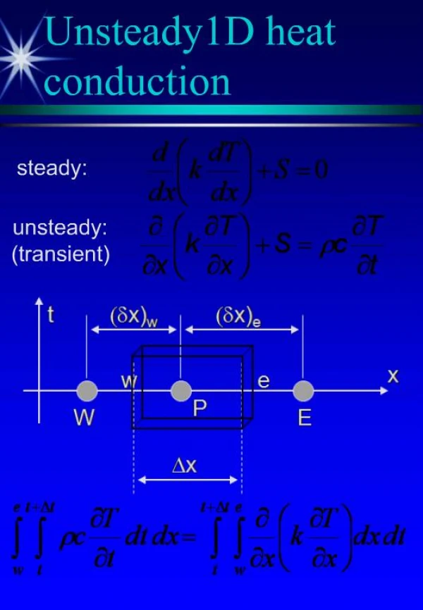
Numerical Methods for Unsteady Heat Transfer • Unsteady heat transfer equation, no generation, constant k, one-dimensional in Cartesian coordinate: • The term on the left hand side of above eq. is the storage term, arising out of accumulation/depletion of heat in the domain under consideration. Note that the eq. is a partial differential equation as a result of an extra independent variable, time (t). The corresponding grid system is shown in fig. on next slide.
t (dx)w (dx)e x e w P W E ∆x Integration over the control volume and over a time interval gives
If the temperature at a node is assumed to prevail over the whole control volume, applying the central differencing scheme, one obtains: Now, an assumption is made about the variation of TP, TE and Twwith time. By generalizing the approach by means of a weighting parameter f between 0 and 1: Repeating the same operation for points E and W,
Upon re-arranging, dropping the superscript “new”, and casting the equation into the standard form ; ; ; ; The time integration scheme would depend on the choice of the parameter f. When f = 0, the resulting scheme is “explicit”; when 0 < f ≤ 1, the resulting scheme is “implicit”; when f = 1, the resulting scheme is “fully implicit”, when f = 1/2, the resulting scheme is “Crank-Nicolson”.
f=0 T TP old f=0.5 TP new f=1 t+Dt t t Variation of T within the time interval ∆t for different schemes Explicit scheme Linearizing the source term as and setting f = 0 For stability, all coefficients must be positive in the discretized equation. Hence,
; ; ; The above limitation on time step suggests that the explicit scheme becomes very expensive to improve spatial accuracy. Hence, this method is generally not recommended for general transient problems. ; Crank-Nicolson scheme Setting f = 0.5, the Crank-Nicolson discretisation becomes:
; For stability, all coefficient must be positive in the discretized equation, requiring ; ; The Crank-Nicolson scheme only slightly less restrictive than the explicit method. It is based on central differencing and hence it is second-order accurate in time. The fully implicit scheme Setting f = 1, the fully implicit discretisation becomes:
General remarks: A system of algebraic equations must be solved at each time level. The accuracy of the scheme is first-order in time. The time marching procedure starts with a given initial field of the scalar 0. The system is solved after selecting time step Δt. For the implicit scheme, all coefficients are positive, which makes it unconditionally stable for any size of time step. Hence, the implicit method is recommended for general purpose transient calculations because of its robustness and unconditional stability.
![Chapter 3: Unsteady State [ Transient ] Heat Conduction](https://cdn1.slideserve.com/2468294/chapter-3-unsteady-state-transient-heat-conduction-dt.jpg)