
Unit 10: Hypothesis Tests
E N D
Presentation Transcript
Significance test outline • Gather data – it won’t fit prevailing theory. Is it different enough to be “significant”? • Formulate H0 (the prevailing theory) and maybe Ha, the “null” and “alternate hypotheses” • Compute a variable (z, t, F, χ2, ...) from data • Compute probability (P-value) that, if H0 is true, test variable would have that value or more extreme • test variable (z or t, vs. one that has only + values) and form of Ha (“z ≥ ?” vs. “z ≥ ? or z ≤ -?”) determine “one-sided” vs. “two-sided” test • If P is small enough (≤ α; usually 5%), result is “(statistically) significant”, and we “reject the null hypothesis”. • We never “accept the null hypothesis” – we just “fail to reject” it. A bit more on this later.
Sig tests we’ll study: • Unit 10: • z-test • t-test (for small samples, n < 25 – but often people speak only of t-tests, even though they are really doing a z-test: t approaches z as n gets bigger) • Unit 11: • 2-sample z-test (special case: difference in avgs of samples from 2 populations) • chi-squared test (for differences in counts in categories) • Quick intros • ANOVA (“analysis of variance”, one-way only; for difference in avgs of samples from several populations) • z-test for nonzeroness of a regr line’s slope • FPP doesn’t approve of this one, but it’s common
Testing % (proportion) • [These are 0-1 boxes.] • H0 implies a population % μ ... • ... which implies σ = √[μ(1- μ)] – use them in computing the P-value
Example: s/l => intermediate? (I) • The African kumquat has short, intermediate and long maturation times. One genetic model says that maturation is controlled by one gene, in two forms: short (s) and long (l), neither dominant – intermediate appears in genotype s/l (or l/s). Suppose some short and some intermediate kumquats are crossed, and of 80 random offspring, 45 are short and 35 intermediate. Does that fit the model?
Normal table z Area(%) z Area(%) z Area(%) z Area(%) z Area(%) 0.0 0.0 0.9 63.19 1.8 92.81 2.7 99.31 3.6 99.968 0.05 3.99 0.95 65.79 1.85 93.57 2.75 99.4 3.65 99.974 0.1 7.97 1 68.27 1.9 94.26 2.8 99.49 3.7 99.978 0.15 11.92 1.05 70.63 1.95 94.88 2.85 99.56 3.75 99.982 0.2 15.85 1.1 72.87 2 95.45 2.9 99.63 3.8 99.986 0.25 19.74 1.15 74.99 2.05 95.96 2.95 99.68 3.85 99.988 0.3 23.58 1.2 76.99 2.1 96.43 3 99.73 3.9 99.99 0.35 27.37 1.25 78.87 2.15 96.84 3.05 99.771 3.95 99.992 0.4 31.08 1.3 80.64 2.2 97.22 3.1 99.806 4 99.9937 0.45 34.73 1.35 82.3 2.25 97.56 3.15 99.837 4.05 99.9949 0.5 38.29 1.4 83.85 2.3 97.86 3.2 99.863 4.1 99.9959 0.55 41.77 1.45 85.29 2.35 98.12 3.25 99.885 4.15 99.9967 0.6 45.15 1.5 86.64 2.4 98.36 3.3 99.903 4.2 99.9973 0.65 48.43 1.55 87.89 2.45 98.57 3.35 99.919 4.25 99.9979 0.7 51.61 1.6 89.04 2.5 98.76 3.4 99.933 4.3 99.9983 0.75 54.67 1.65 90.11 2.55 98.92 3.45 99.944 4.35 99.9986 0.8 57.63 1.7 91.09 2.6 99.07 3.5 99.953 4.4 99.9989 0.85 60.47 1.75 91.99 2.65 99.2 3.55 99.961 4.45 99.9991
Example: morning sickness => girl? • (Adapted from Syracuse Post-Standard, 99/12/9, p A-16) Swedish scientists examined all births in Sweden between ’87 and ’95, and found that 51% were girls. But of 5900 women who had extreme morning sickness during first trimester, 56% had girls. Does extreme morning sickness in first trimester mean a girl is more likely?
Testing μ of numerical variable • [These are boxes of multivalued tickets.] • H0 usually implies only μ; • use sample s to approximate population σ in computing P-value • bootstrapping
Example: vit A => smart rat? • Testing effect of vitamin A on rat learning: 200 rats paired at random. One of each pair gets vit A supplements, then both run a maze. The quantity untreated rat’s time – treated rat’s time has an avg of 1.1 sec, with SD of 5 sec. Did vit A help rats to learn to run the maze? Or was it just chance variation?
Normal table z Area(%) z Area(%) z Area(%) z Area(%) z Area(%) 0.0 0.0 0.9 63.19 1.8 92.81 2.7 99.31 3.6 99.968 0.05 3.99 0.95 65.79 1.85 93.57 2.75 99.4 3.65 99.974 0.1 7.97 1 68.27 1.9 94.26 2.8 99.49 3.7 99.978 0.15 11.92 1.05 70.63 1.95 94.88 2.85 99.56 3.75 99.982 0.2 15.85 1.1 72.87 2 95.45 2.9 99.63 3.8 99.986 0.25 19.74 1.15 74.99 2.05 95.96 2.95 99.68 3.85 99.988 0.3 23.58 1.2 76.99 2.1 96.43 3 99.73 3.9 99.99 0.35 27.37 1.25 78.87 2.15 96.84 3.05 99.771 3.95 99.992 0.4 31.08 1.3 80.64 2.2 97.22 3.1 99.806 4 99.9937 0.45 34.73 1.35 82.3 2.25 97.56 3.15 99.837 4.05 99.9949 0.5 38.29 1.4 83.85 2.3 97.86 3.2 99.863 4.1 99.9959 0.55 41.77 1.45 85.29 2.35 98.12 3.25 99.885 4.15 99.9967 0.6 45.15 1.5 86.64 2.4 98.36 3.3 99.903 4.2 99.9973 0.65 48.43 1.55 87.89 2.45 98.57 3.35 99.919 4.25 99.9979 0.7 51.61 1.6 89.04 2.5 98.76 3.4 99.933 4.3 99.9983 0.75 54.67 1.65 90.11 2.55 98.92 3.45 99.944 4.35 99.9986 0.8 57.63 1.7 91.09 2.6 99.07 3.5 99.953 4.4 99.9989 0.85 60.47 1.75 91.99 2.65 99.2 3.55 99.961 4.45 99.9991
Effect of sample size • Valesky vs. Brown: Both surveys below say 54% for V., so for CI, EV of sample % is .54. And for sig test: H0: p = 0.5, Ha: p > 0.5. • n = 100: For CI, SE = √[.54(.46)/100] = .05, so 54% ± 10%. For sig test, SE = √[.5(.5)/100] = .05, so P(% ≥ .54) = P(z ≥ (.54-.5)/.05 = .8) = 21% • n = 1600: For CI, SE = √[.54(.46)/1600] = .0125, so 54% ± 2.5%. For sig test, SE = √[.5(.5)/1600] = .0125, so P(% ≥ .54) = P(z ≥ (.54-.5)/.0125 = 3.2) = .07%
Recall t-test for small samples • Use when n ≤ 25 . • Differences: • In tests of numerical variable (not %), use sample SD, s or SD+, not σ . • Use t-table with proper degrees of freedom: df = n-1 [table set up differently from z] • Roughly bell-shaped curves, less area (height) in center, more in tails than normal • As df grows, less in tails, more in center • History: W. S. Gossett (1876-1936) invented t-distribution because small samples were more variable than z-distribution. Working at Guinness brewery, he published as “Student” so the competition wouldn’t realize his work was useful.
Example: s/l => intermediate? (II) • The African kumquat has short, intermediate and long maturation times. One genetic model says that maturation is controlled by one gene, in two forms: short (s) and long (l), neither dominant – intermediate appears in genotype s/l (or l/s). Suppose some short and some intermediate kumquats are crossed, and of 20 random offspring, 7 are short and 13 intermediate. Does that fit the model?
Example: School uniforms raise GPA? Data from online survey, S’06: GPA for all respondents averaged 3.086, but 25 who wore uniforms in HS averaged 3.224, with SD of .439. Do school uniforms raise the students’ GPA’s?
Example: cold drug • New drug for cold symptoms; does it last more than 2 hr? 15 subjects with colds get dosed, find that it wears off after 2.2 hr, with s = .3 hr. Does drug’s effect avg more than 2 hr (in whole population)?
Sig tests vs. confidence intvls • Many authors prefer CI’s • because they give all plausible values • CI equivalent to 2-sided sig test (almost: In t-test for %, s ≠ σ) • Ex: s/l => intermediate? (I): • Sig test: 45 of 80 is not significantly different from H0’s predicted 40. • CI: 95% CI for count of int maturers is 45 ± 2√[(.5625)(.4375)]√80 : 45 ± 8.9 • which includes 40 • Ex: cold drug: • Sig test: 2.2 hr, with s = .3 hr, is significantly larger than 2 hr • CI: 95% CI for time the new one lasts is 2.2 ± 2.131(.3/√(15)) : 2.2 ± .17 hr • which excludes 2 hr
Sgn test: Are x,y really related? • Regression line for data points in a sample is only an approximation to the best linear relation in the population between each x-value and the avgµy of all the y-values at that x: µy = α + βx , where α, β are the intercept and slope for the population relation. • Are populations x,y really related, i.e., is β ≠ 0? • Sgn test: H0: β = 0, t = (n-2) r/√[1-r2], df = n-2 • Some statisticians, like our authors, disapprove of this test: values of b don’t follow t-distribution • very likely to be significant -- n-2 is often big
Example: H0: β = 0 t = (4-2) (.434)/ √[1-(.434)2] ≈ .963 , df = 4-2 = 2 P(t ≥ .963 or ≤ -.963) is not less than 5%, so we fail to reject the null hypothesis: x and y are not related.