Chapter 16 Single-Population Hypothesis Tests
300 likes | 538 Vues
Chapter 16 Single-Population Hypothesis Tests. Hypothesis Tests. A statistical hypothesis is an assumption about a population parameter. There are two types of statistical hypotheses.

Chapter 16 Single-Population Hypothesis Tests
E N D
Presentation Transcript
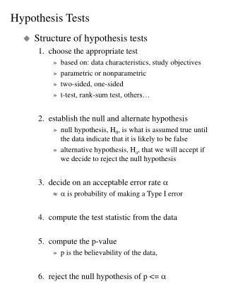
Hypothesis Tests • A statistical hypothesis is an assumption about a population parameter. • There are two types of statistical hypotheses. • Null hypothesis -- The null hypothesis, H0, represents a theory that has been put forward, either because it is believed to be true or because it is to be used as a basis for argument, but has not been proved. • Alternative hypothesis (Research hypothesis) -- The alternative hypothesis, H1, is a statement of what a statistical hypothesis test is set up to establish.
Hypothesis Tests Examples • Trials • H0: The person is innocent • H1: The person is guilty • Soda • H0: = 12 oz • H1: < 12 oz
Hypothesis Tests • Test Statistics -- the random variable X whose value is tested to arrive at a decision. • Critical values-- the values of the test statistic that separate the rejection and non-rejection regions. • Rejection Region -- the set of values for the test statistic that leads to rejection of H0 • Non-rejection region -- the set of values not in the rejection region that leads to non-rejection of H0
Errors in Hypothesis Tests • (Significance level): Probability of making Type I error • : Probability of making Type II error • 1-: Power of Test (Probability of rejecting H0 when H0 is false)
Hypothesis TestsExamples Two-tailed test: According to the US Bureau of the Census, the mean family size was 3.17 in 1991. An economist wants to check whether or not this mean has changed since 1991. H0: = 3.17 H1: 3.17 C2 C1 1- /2 /2 =3.17 Rejection Region Rejection Region Non-rejection Region
Hypothesis TestsExamples Left-tailed test: A soft-drink company claims that, on average, its cans contain 12 oz of soda. Suppose that a consumer agency wants to test whether the mean amount of soda per can is less than 12 oz. H0: = 12 H1: < 12 C 1- =12 Rejection Region Non-rejection Region
Hypothesis TestsExamples Right-tailed test: According to the US Bureau of the Census, the mean income of all households was $37,922 in 1991. Suppose that we want to test whether the current mean income of all households is higher than $37,922. C H0: = 37922 H1: > 37922 1- =37922 Rejection Region Non-rejection Region
Hypothesis TestsRejection Region Approach • Select the type of test and check the underlying conditions • State the null and alternative hypotheses • Determine the level of significance • Calculate the test statistics • Determine the critical values and rejection region • Check to see whether the test statistic falls in the rejection region • Make decision
Hypothesis TestsP-Value Approach • Select the type of test and check the underlying conditions • State the null and alternative hypotheses • Determine the level of significance • Calculate the p-value (the smallest level of significance that would lead to rejection of the null hypothesis H0 with given data) • Check to see if the p-value is less than • Make decision
Testing Hypothesis on the Meanwith Variance Known (Z-Test) • Null Hypothesis: H0: = 0 • Test statistic:
Testing Hypothesis on the Meanwith Variance Known (Z-Test)– Example 16.1 • Claim: Burning time at least 3 hrs • n=42, =0.23, =.10 • Null Hypothesis: H0: 3 • Alt. Hypothesis: H1: < 3 • Test statistic: • Rejection region: z= z.10=-1.282 • P-value = P(z<-1.13) = .1299 • Fail to reject H0 C .9 .1 =3 Rejection Region Non-rejection Region -1.282
Testing Hypothesis on the Meanwith Variance Known (Z-Test)– Example 16.2 • Claim: Width =38” • n=80, =0.098, =.05 • Null Hypothesis: H0: = 38 • Alt. Hypothesis: H1: 38 • Test statistic: • Rejection region: z/2= z.025=-1.96 • z1-/2= z.975= 1.96 • P-value = P(z>1.825)+P(z<-1.825) = .0679 • Fail to reject H0 C2 C1 .95 .025 .025 =38 Rejection Region Rejection Region Non-rejection Region 1.96 -1.96
Type II Error and Sample Size • Increasing sample size could reduce Type II error C2 C1 1- = 0 = 0+ Non-rejection Region
Testing Hypothesis on the Meanwith Variance Known (Z-Test)– Example • Claim: Burning rate = 50 cm/s • n=25, =2, =.05 • Null Hypothesis: H0: = 50 • Alt. Hypothesis: H1: 50 • Test statistic: • Rejection region: z/2= z.025=-1.96 • z1-/2= z.975= 1.96 • P-value = P(z>3.25)+P(z<-3.25) = .0012 • Reject H0 C2 C1 .95 .025 .025 =50 Rejection Region Rejection Region Non-rejection Region 1.96 -1.96
Type II Error and Sample Size - Example • Claim: Burning rate = 50 cm/s • n=25, =2, =.05, =.10 • Hypothesis: H0: = 50; H1: 50 • If = 51 C2 C1 1- = 0 = 0+ Non-rejection Region
Testing Hypothesis on the Meanwith Variance Unknown (t-Test) • Null Hypothesis: H0: = 0 • Test statistic:
Testing Hypothesis on the Meanwith Variance Unknown (t-Test)– Example 16.3 • Claim: Length =2.5” • n=49, s=0.021, =.05 • Null Hypothesis: H0: = 2.5 • Alt. Hypothesis: H1: 2.5 • Test statistic: • Rejection region: t.025,48= 2.3139 • P-value = 2*P(t>3.33)= .0033 • Reject H0 C2 C1 .95 .025 .025 =2.5 Rejection Region Rejection Region Non-rejection Region 2.31 -2.31
Testing Hypothesis on the Meanwith Variance Unknown (t-Test)– Example 16.4 • Claim: Battery life at least 65 mo. • n=15, s=3, =.05 • Null Hypothesis: H0: 65 • Alt. Hypothesis: H1: < 65 • Test statistic: • Rejection region: -t.05, 14=-2.14 • P-value = P(t<-2.582) = .0109 • Reject H0 C .95 .05 =65 Rejection Region Non-rejection Region -2.14
Testing Hypothesis on the Meanwith Variance Unknown (t-Test)– Example 16.5 • Claim: Service rate = 22 customers/hr • n=18, s=4.2, =.01 • Null Hypothesis: H0: = 22 • Alt. Hypothesis: H1: > 22 • Test statistic: • Rejection region: t.01,17= 2.898 • P-value = P(t>1.717)= .0540 • Fail to reject H0 C .99 .01 =22 Rejection Region Non-rejection Region 2.31
Testing Hypothesis on the Median • Null Hypothesis: H0: = 0 • Test statistic: SH = No. of observations greater than 0 • SL = No. of observations less than 0
Testing Hypothesis on the Median– Example 16.6 • Claim: Median spending = $67.53 • n=12, =.10 • Null Hypothesis: H0: = 67.53 • Alt. Hypothesis: H1: > 67.53 • Test statistic: SH = 9, SL = 3 • P-value = P(x9)= P(x=9)+P(x=10)+P(x=11)+P(x=12) • =.0730 • Reject H0
Testing Hypothesis on the Variance of a Normal Distribution • Null Hypothesis: H0: 2 = 02 • Test statistic:
Testing Hypothesis on the Variance– Example • Claim: Variance 0.01 • s2=0.0153, n=20, =.05 • Null Hypothesis: H0: 2 = .01 • Alt. Hypothesis: H1: 2 > .01 • Test statistic: • Rejection region: 2.05,19= 30.14 • p-value = P(2 >29.07)=0.0649 • Fail to reject H0 C .95 .05 Rejection Region Non-rejection Region 30.14
Testing Hypothesis on the Population Proportion • Null Hypothesis: H0: p = p0 • Test statistic:
Testing Hypothesis on the Population Proportion – Example 16.7 • Claim: Market share = 31.2% • n=400, =.01 • Null Hypothesis: H0: p = .312 • Alt. Hypothesis: H1: p .312 • Test statistic: • Rejection region: z/2= z.005=-2.576 • z1-/2= z.995= 2.576 • P-value = P(z>.95)+P(z<-.95) = .3422 • Fail to reject H0 C2 C1 .99 .005 .005 =.312 Rejection Region Rejection Region Non-rejection Region 2.576 -2.576
Testing Hypothesis on the Population Proportion – Example 16.8 • Claim: Defective rate 4% • n=300, =.05 • Null Hypothesis: H0: p = .04 • Alt. Hypothesis: H1: p > .04 • Test statistic: • Rejection region: z1-= z.95= 1.645 • P-value = P(z>2.65) = .0040 • Reject H0 C .95 .05 =.04 Rejection Region Non-rejection Region 1.645