Hypothesis Tests Regarding a Parameter – Single Mean & Single Proportion
Hypothesis Tests Regarding a Parameter – Single Mean & Single Proportion. Overview. This is the other part of inferential statistics, hypothesis testing Hypothesis testing and estimation are two different approaches to two similar problems


Hypothesis Tests Regarding a Parameter – Single Mean & Single Proportion
E N D
Presentation Transcript
Hypothesis Tests Regarding a Parameter – Single Mean & Single Proportion
Overview • This is the other part of inferential statistics, hypothesistesting • Hypothesis testing and estimation are two different approaches to two similar problems • Estimation is the process of using sample data to estimate the value of a population parameter • Hypothesis testing is the process of using sample data to test a claim about the value of a population parameter
The Language of Hypothesis Testing
Hypothesis Testing • The environment of our problem is that we want to test whether a particular claim is believable, or not • The process that we use is called hypothesistesting • This is one of the most common goals of statistics
Hypothesis Testing • Hypothesis testing involves two steps • Step 1 – to state what we think is true • Step 2 – to quantify how confident we are in our claim • The first step is relatively easy • The second step is why we need statistics
Hypothesis Testing • We are usually told what the claim is, what the goal of the test is • Now similar to estimation in the previous unit discussed, we will again use the material regarding the sampling distribution of the sample mean to quantify how confident we are in our claim
Example • An example of what we want to quantify • A car manufacturer claims that a certain model of car achieves 29 miles per gallon • To test for the claim, we then test some number of cars • We calculate the sample mean … it is 27 • Is 27 miles per gallon consistent with the manufacturer’s claim? How confident are we that the manufacturer has significantly overstated the miles per gallon achievable?
Example • How confident are we that the gas economy is definitely less than 29 miles per gallon? • We would like to make either a statement “We’re pretty sure that the mileage is less than 29 mpg” or “It’s believable that the mileage is equal to 29 mpg”
Level of Significance • A hypothesis test for an unknown parameter is a test of a specific claim • Compare this to a confidence interval which gives an interval of numbers, not a “believe it” or “don’t believe it” answer • The levelofsignificance reflects the confidence we have in our conclusion
Null Hypothesis • How do we state our claim? • Our claim • Is the statement to be tested • Is called the nullhypothesis • Is written as H0 (and is read as “H-naught”)
Alternative Hypothesis • How do we state our counter-claim? • Our counter-claim • Is the opposite of the statement to be tested • Is called the alternativehypothesis • Is written as H1 (and is read as “H-one”)
Two-tailed Test • There are different types of null hypothesis / alternative hypothesis pairs, depending on the claim and the counter-claim • One type of H0 / H1 pair, called a two-tailed (or two-sided)test, tests whether the parameter is either equal to, versus not equal to, some value • H0: parameter = some value • H1: parameter ≠ some value
Example • An example of a two-tailed test • A bolt manufacturer claims that the diameter of the bolts average 10 mm • H0: Diameter = 10 • H1: Diameter ≠ 10 • An alternative hypothesis of “≠ 10” is appropriate since • A sample diameter that is too high may be a problem • A sample diameter that is too low may also be a problem That is, we may reject the claim under the H0 , if the sample value is either too high or too low • Thus this is a two-tailed test
Left-tailed Test • Another type of pair, called a left-tailedtest, tests whether the parameter is either equal to, versus less than, some value • H0: parameter = some value (This actually means Parameter some value) • H1: parameter < some value Note: Equality sign appears only in the null hypothesis.
Example • An example of a left-tailed test • A car manufacturer claims that the mpg of a certain model car is at least 29.0 • H0: MPG = 29.0 (In fact, this does not mean MPG is only 29.0. it means MPG 29.0 ) • H1: MPG < 29.0 • An alternative hypothesis of “< 29” is appropriate since • A mpg that is too low is a problem • A mpg that is too high is not a problem That is, we reject the claim under the H0, if the sample mpg observed is too low, much lower than 29. • Thus this is a left-tailed test. (The side of the tail depends on the direction under H1 which tends to support a lower value of MPG. And a lower value is located on the left of a higher value on a number line. Note: By convention, we always only put the equality sign for the claim in H0 , even though it should be MPG 29.0. This is because we can tell the actual direction of the inequality sign under H0 by just looking at the sign in H1 (H0 is the opposite of H1. Since MPG is less than 29 in H1, MPG will be no less than 29 under H0.)
Right-tailed Test • Another third type of pair, called a right-tailedtest, tests whether the parameter is either equal to, versus greater than, some value • H0: parameter = some value (This actually means parameter Some value.) • H1: parameter > some value Note: Equality sign appears only under the null hypothesis H0
Example • An example of a right-tailed test • A bolt manufacturer claims that the defective rate of their product is at most 1 part in 1,000 • H0: Defect Rate = 0.001 • H1: Defect Rate > 0.001 • An alternative hypothesis of “> 0.001” is appropriate since • A defect rate that is too low is not a problem • A defect rate that is too high is a problem That is, higher defective rate observed tends to be in favor of H1, , but againstH0. • Thus this is a right-tailed test
One-tailed and Two-tailed Tests • A comparison of the three types of tests • The null hypothesis • We believe that this is true • The alternative hypothesis
Example 1 • A manufacturer claims that there are at least two scoops of cranberries in each box of cereal • What would be a problem? • The parameter to be tested is the number of scoops of cranberries in each box of cereal • If the sample mean is too low, that is a problem • If the sample mean is too high, that is not a problem • This is a left-tailed test • The “bad case” is when there are too few
Example 2 • A manufacturer claims that there are exactly 500 mg of a medication in each tablet • What would be a problem? • The parameter to be tested is the amount of a medication in each tablet • If the sample mean is too low, that is a problem • If the sample mean is too high, that is a problem too • This is a two-tailed test • A “bad case” is when there are too few
Example 3 • A manufacturer claims that there are at most 8 grams of fat per serving • What would be a problem? • The parameter to be tested is the number of grams of fat in each serving • If the sample mean is too low, that is not a problem • If the sample mean is too high, that is a problem • This is a right-tailed test • The “bad case” is when there are too many
Reject or Not to reject H0 • There are two possible results for a hypothesis test • If we believe that the null hypothesis could be true, this is called notrejectingthenullhypothesis • Note that this is only “we believe … could be” • If we are pretty sure that the null hypothesis is not true, so that the alternative hypothesis is true, this is called rejectingthenullhypothesis • Note that this is “we are pretty sure that … is”
Decision Errors • In comparing our conclusion (not reject or reject the null hypothesis) with reality, we could either be right or we could be wrong • When we reject (and state that the null hypothesis is false) but the null hypothesis is actually true • When we not reject (and state that the null hypothesis could be true) but the null hypothesis is actually false • These would be undesirable errors
Type I and II Errors • A summary of the errors is • We see that there are four possibilities … in two of which we are correct and in two of which we are incorrect
Type I and II Errors • When we reject the null hypothesis (and state that the null hypothesis is false) but the null hypothesis is actually true … this is called a TypeIerror • When we do not reject the null hypothesis (and state that the null hypothesis could be true) but the null hypothesis is actually false … this called a TypeIIerror • In general, Type I errors are considered the more serious of the two
Example • A very good analogy for Type I and Type II errors is in comparing it to a criminal trial • In the US judicial system, the defendant “is innocent until proven guilty” • Thus the defendant is presumed to be innocent • The null hypothesis is that the defendant is innocent • H0: the defendant is innocent
Example (continued) • If the defendant is not innocent, then • The defendant is guilty • The alternative hypothesis is that the defendant is guilty • H1: the defendant is guilty • The summary of the set-up • H0: the defendant is innocent • H1: the defendant is guilty
Example (continued) • Our possible conclusions • Reject the null hypothesis • Go with the alternative hypothesis • H1: the defendant is guilty • We vote “guilty” • Do not reject the null hypothesis • Go with the null hypothesis • H0: the defendant is innocent • We vote “not guilty” (whichisnotthesameasvotinginnocent! Voting “not guilty” does not prove the defendant is innocent, we just do not have enough evidence to against the defendant.)
Example (continued) • A Type I error • Reject the null hypothesis • The null hypothesis was actually true • We voted “guilty” for an innocent defendant • A Type II error • Do not reject the null hypothesis • The alternative hypothesis was actually true • We voted “not guilty” for a guilty defendant
Example (continued) • Which error do we try to control? • Type I error (sending an innocent person to jail) • The evidence was “beyond a reasonable doubt” • We must be pretty sure • Very bad! We want to minimize this type of error • A Type II error (letting a guilty person go) • The evidence wasn’t “beyond a reasonable doubt” • We weren’t sure enough • If this happens … well … it’s not as bad as a Type I error (according to the US system)
Reject or Not to reject H0 • “Innocent” versus “Not Guilty” • This is an important concept • Innocent is not the same as not guilty • Innocent – the person did not commit the crime • Not guilty – there is not enough evidence to convict … that the reality is unclear • To not reject the null hypothesis – doesn’t mean that the null hypothesis is true – just that there isn’t enough evidence to reject
Summary • A hypothesis test tests whether a claim is believable or not, compared to the alternative • We test the null hypothesis H0 versus the alternative hypothesis H1 • If there is sufficient evidence to conclude that H0 is false, we reject the null hypothesis • If there is insufficient evidence to conclude that H0 is false, we do not reject the null hypothesis
Hypothesis Tests for a Population Mean Assuming the Population Standard Deviation is Known
Learning Objectives • Understand the logic of hypothesis testing • Test hypotheses about a population mean with σ known using the classical approach • Test hypotheses about a population mean with σ known using P-values approach • Test hypotheses about a population mean with σ known using confidence intervals approach
Decision Rule • Hypothesis test is to set up a decision rule for the sample data to reject or not to reject the null hypothesis • How do we quantify “unlikely” the null hypothesis is true? • What is the exact procedure to get to a “do not reject” or “reject” conclusion?
Methods of Hypothesis Testing • There are three equivalent ways to perform a hypothesis test • They will reach the same conclusion • The methods • The classical approach • The P-value approach • The confidence interval approach
Methods of Hypothesis Testing • The classical approach • If the sample value observed is too many standard deviations away from the true value claimed under H0, then it must be too unlikely H0 is true • The P-value approach • If the probability of the sample value being that far away is small, then it must be too unlikely H0 is true • The confidence interval approach • If we are not sufficiently confident that the parameter is likely enough, then it must be too unlikely • Don’t worry … we’ll be explaining more
Basic Steps to Test the Hypothesis Step 1: We set up the null hypothesis that the actual mean μ is equal to a value μ0 and the alternative hypothesis Step 2: We set up a criterion (to reject H0) • A criterion that quantifies “unlikely” the null hypothesis that the actual mean μ being equal to a specified value of μ0 is true. That is, the actual mean is unlikely to be equal to μ0
Collect Sample Data • The three methods all need information • We run an experiment • We collect the data • We calculate the sample mean • The three methods all make the same assumptions to be able to make the statistical calculations • That the sample is a simple random sample • That the sample mean has a normal distribution
Choose a Test Statistic • We first assume that the population standard deviation σis known • We use a sample estimate, for instance, a sample mean to test for the population parameter - the population mean μ • We can apply our techniques if either • The population has a normal distribution • Our sample size n is large (n≥ 30) • In those cases, the distribution of the sample mean is normal with mean μ and standard deviation σ / √ n
Check the criterion for Unlikely • The three methods all compare the observed results with the criterion that quantifies “unlikely”: • Classical – how many standard deviations • P-value – the size of the probability • Confidence interval – inside or outside the interval • If the results are unlikely based on these criterion, we reject the claim under the null hypothesis.
Statistical Significance • The three methods all conclude similarly • We do not reject the null hypothesis, or • We reject the null hypothesis • When we reject the null hypothesis, we say that the result is statistically significant
Perform Hypothesis Testing • We now will cover how each of the • Classical • P-value, and • Confidence interval approaches will show us how to conclude whether the result is statistically significant or not
Test hypotheses about a population mean with σ known using the classical approach
The Classical Approach • We compare the sample mean to the hypothesized population mean μ0 • Measure the difference in units of standard deviations, which is called the test statistic: • A lot of standard deviations is far … few standard deviations is not far • Just like using a general normal distribution
α Level of Significance • How far is too far? • For example, we can set α = 0.05 as the size of “unlikely”, so-called “the level of significance” • “Unlikely” means that this difference occurs with probability α = 0.05 of the time, or less under the null hypothesis • This concept applies to two-tailed tests, left-tailed tests, and right-tailed tests Note: αis often determined subjectively before the experiment. It sets up a rule to reject the null hypothesis. So, it is also the size of the risk for committing a type I error of rejecting the null hypothesis by mistake.