Inference for proportions - Inference for a single proportion

1. Inference for proportions- Inference for a single proportion IPS chapter 8.1 © 2006 W.H. Freeman and Company

2. Objectives (IPS chapter 8.1) Inference for a single proportion • Conditions for inference on p • Large-sample confidence interval for p • “Plus four” confidence interval for p • Significance test for a proportion • Sample size for a desired margin of error

3. Sampling distribution of p^ — reminder The sampling distribution of a sample proportion is approximately normal (normal approximation of a binomial distribution) when the sample size is large enough.

4. Conditions for inference on p Assumptions: • The data used for the estimate are a random sample from the population studied. • The population is at least 10 times as large as the sample used for inference. This ensures that the standard deviation of is close to • The sample size n is large enough that the sampling distribution can be approximated with a normal distribution. “How large a sample size is required” depends in part on the value of p and the test conducted. Otherwise, rely on the binomial distribution.

5. C mm −Z* Z* Large-sample confidence interval for p For a random sample of size n drawn from a large population and with sample proportion calculated from the data, an approximate level C(=1-α) confidence interval for p is: Use this method when n≥25, and C is the area under the standard normal curve between −z* and z*.

6. Medication side effects Arthritis is a painful, chronic inflammation of the joints. An experiment on the side effects of pain relievers examined arthritis patients to find the proportion of patients who suffer side effects. Suppose 23 out of 440 arthritis patients suffer side effects. What are some side effects of ibuprofen? Serious side effects (seek medical attention immediately): Allergic reaction (difficulty breathing, swelling, or hives), Muscle cramps, numbness, or tingling, Ulcers (open sores) in the mouth, Rapid weight gain (fluid retention), Seizures, Black, bloody, or tarry stools, Blood in your urine or vomit, Decreased hearing or ringing in the ears, Jaundice (yellowing of the skin or eyes), or Abdominal cramping, indigestion, or heartburn, Less serious side effects (discuss with your doctor): Dizziness or headache, Nausea, gaseousness, diarrhea, or constipation, Depression, Fatigue or weakness, Dry mouth, or Irregular menstrual periods

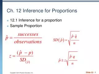
7. Our goal is to calculate a 90% confidence interval for the population proportion of arthritis patients who suffer some “adverse symptoms.” What is the sample proportion ? What is the sampling distribution for the proportion of arthritis patients with adverse symptoms for samples of 440? For a 90% confidence level, z* = 1.645. Using the large sample method, we calculate a margin of error m:  With 90% confidence level, between 2.9% and 7.5% of arthritis patients experience some adverse symptoms.

8. We can find this C.I. by the following R command. > prop.test(23, 440, conf.level = 0.9) 1-sample proportions test with continuity correction data: 23 out of 440, null probability 0.5 X-squared = 351.0205, df = 1, p-value < 2.2e-16 alternative hypothesis: true p is not equal to 0.5 90 percent confidence interval: 0.03644228 0.07392657 sample estimates: p 0.05227273

9. Because we have to use an estimate of p to compute the margin of error, confidence intervals for a population proportion are not very accurate. Specifically, we tend to be incorrect more often than the confidence level would indicate. But there is no systematic amount (because it depends on p). Use with caution!

10. “Plus four” confidence interval for p We need an adjustment to produce more accurate confidence intervals. We act as if we had four additional observations, two being successes and two being failures. Thus, the new sample size is n + 4 and the count of successes is X + 2. The “plus four” estimate of p is: And an approximate level C(=1-α) confidence interval is:

11. We now use the “plus four” method to calculate the 90% confidence interval for the population proportion of arthritis patients who suffer some “adverse symptoms.” What is the value of the “plus four” estimate of p? An approximate 90% confidence interval for p using the “plus four” method is: • With 90% confidence level, between 3.8% and 7.4% of arthritis patients • experience some adverse symptoms.

12. Significance test for p The sampling distribution for is approximately normal for large sample sizes and its shape depends solely on p and n. Thus, we can easily test the null hypothesis: H0: p = p0 (a given value we are testing). If H0 is true, the sampling distribution is known  The likelihood of our sample proportion given the null hypothesis depends on how far from p0 our is in units of standard deviation. This is valid when and .

13. P-values and one or two sided hypotheses—reminder And as always, if the p-value is smaller than the chosen significance level a, then the difference is statistically significant and we reject H0.

14. A national survey on restaurant employees found that 75% said that work stress had a negative impact on their personal lives. You investigate a restaurant chain to see if the proportion of all their employees negatively affected by work stress differs from the national proportion p0 = 0.75. H0: p = 0.75 vs. Ha: p≠ 0.75 (2 sided alternative) In your random sample of 100 employees, you find that 68 answered “Yes” when asked, “Does work stress have a negative impact on your personal life?” Since n∙p0 =100 × 0.75 = 75 and n∙(1-p0 )= 100 × 0.25 = 25, we can use a normal approximation. The test statistic is:

15. From Table A we find the area to the left of z 1.62 is 0.9474. So, P-value= 2P(Z ≥ 1.62)= 2∙pnorm(1.62,0,1,lower.tail=F)=0.1052 ≈0.11, Which is larger than α.  The chain restaurant data are not significantly different from the national survey results (pˆ= 0.68, z = 1.62, P = 0.11).

16. We can test “H0: p = p0 = 0.75 vs. Ha: p≠ 0.75” by the following R command. > prop.test(68, 100, 0.75, alternative="two.sided") 1-sample proportions test with continuity correction data: 68 out of 100, null probability 0.75 X-squared = 2.2533, df = 1, p-value = 0.1333 alternative hypothesis: true p is not equal to 0.75 95 percent confidence interval: 0.5782080 0.7677615 sample estimates: p 0.68

17. Sample size for a desired margin of error You may need to choose a sample size large enough to achieve a specified margin of error. It can be done by the following formula: However, because is a function of the sample size n, this process requires that you guess a likely value for . Note that is usually guessed as 1/2. Therefore, n can be determined by the following formula: The margin of error for this n will be less than or equal to m .

18. What sample size would we need in order to achieve a margin of error no more than 0.01 for a 90% confidence interval for the population proportion of arthritis patients who suffer some “adverse symptoms.” For a 90% confidence level, z* = 1.645.  To obtain a margin of error no more than 1%, we would need a sample size n of at least 6766 arthritis patients.