Download

1 / 33
330 likes | 563 Vues
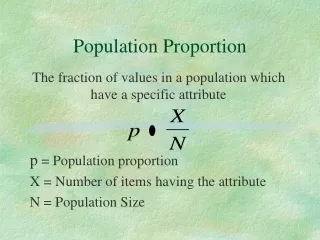
Inference for a Single Population Proportion ( p ). ^. p = estimate of population proportion p = proportion of sample having a specified attribute = . x n. where n = sample size and x = the observed number of “successes” in the sample.

E N D
^ p = estimate of population proportionp = proportion of sample having a specified attribute = x n where n = sample size and x = the observed number of “successes” in the sample Sampling Distribution of the Sample Proportion Sample Proportion
For larger samples, the sampling distribution of the sample proportion is approximately normal. Sampling Distribution of the Sample Proportion The histograms below show the estimated sampling distribution of the sample proportion based upon 1000 samples of the drawn for the given sample size (n).
Sampling Distribution of the Sample Proportion Sampling Distribution of • Provided n is “sufficiently large”, the sampling distribution is normal, generally • The mean of the sampling distribution isp = true population proportion • Standard deviation of the sampling distribution or the standard error of sample proportion is given by: * 5 is also used.
Effect Size Implications for Inference(n “large”) CI for Population Proportion (p) Test Statistic (Ho: p = po) z-values from standard normal90% = 1.64595% = 1.96099% = 2.578
P-value P-value 0 z z 0 Hypothesis Testing for a Population Proportion (p) Null HypothesisHo: p = po Alternative Hypotheses p-value (upper-tailed) (lower-tailed)
z 0 - z Hypothesis Testing for a Population Proportion (p) Null HypothesisHo: p = po Alternative Hypotheses p-value (two-tailed) For two-tailed tests in general it is preferable to simply construct a confidence interval for the parameter of interest and see if the hypothesized value under the null hypothesis is contained in the CI. If it is we fail to reject Ho and if it is not then we reject Ho.
Example: Treatment of Kidney Cancer • Historically, one in five kidney cancer patients survive 5 years past diagnosis, i.e. 20%. • An oncologist using an experimental therapy treats n = 40 kidney cancer patients and 16 of them survive at least 5 years. • Is there evidence that patients receiving the experimental therapy have a higher 5-year survival rate?
Step 1: Formulate Hypotheses p = the proportion of kidney cancer patients receiving the experimental therapy that survive at least 5 years. Step 2: Determine test criteria Choose a = .05 (may want to consider smaller?)Use large sample test ? Definitely questionable as we have… np = (40)(.20) = 8 > 5 and n(1-p) = (40)(.80) = 32 > 5
Step 3: Collect data and compute test statistic The observed 5-yr. survival rate for kidney cancer patients undergoing the experimental therapy is 3.16 standard errors above the historical rate!
P-value = .0008 0 z = 3.16 Step 4: Compute p-value It is highly unlikely we would obtain a 40% 5-yr. survival rate in our sample, if in fact the 5-yr. survival rate for the population of patients treated with the experimental therapy was truly 20%. Step 5: Make Decision and Interpret We have very strong evidence to suggest the 5-year survival rate for kidney cancer patients undergoing the experimental therapy is greater than the current 5-yr. survival rate of 20% (p = .0008).
Step 6: Quantify significant results Confidence Interval Effect Size
Baseline proportion is the proportion under the null hypothesis (.20 or 20% here) Difference to detect is the absolute difference between p under alternative and p under null (i.e., .40 - .20 = .20) Power is calculated once sample size and difference information is entered (here, Power = .935). For power use software Power Calculation
For a difference of .20Power = .935 as seen on previous slide Power Curve for n = 40 and po = .20
Sample Size and CI’s for p • Suppose we wish to estimate p using a 95% CI and have a margin of error of 3%. What sample size do we need to use? • Recall the CI for p is given by: MARGIN OF ERROR (E)
Sample Size and CI’s for p • Here for a 95% CI we want E = .03 or 3% • After some wonderful algebraic manipulation • Oh, oh! We don’t know p-hat !! • “Guesstimate” • Use p-hat from pilot or prior study. • Largest n we would ever need comes when p-hat = .50.
Sample Size and CI’s for p • Informed approach • Conservative approach (i.e. worst case scenario) Standard normal values90% = 1.64595% = 1.96099% = 2.578
Sample Size and CI’s for p • Original Question: Suppose we wish to estimate p using a 95% CI and have a margin of error of 3%. What sample size do we need to use? • Assume that we estimate the 5 yr. survival rate for a new kidney cancer therapy, and we know historical that it this survival rate is around 20%. • Using informed approach
Sample Size and CI’s for p • Original Question: Suppose we wish to estimate p using a 95% CI and have a margin of error of 3%. What sample size do we need to use? • Assume that we estimate the 5 yr. survival rate for a new kidney cancer therapy, and we know historical that it this survival rate is around 20%. • Using conservative approach This is why in media polls you they usually report a sampling error of + 3% and that the poll was based on a sample of n = 1000 individuals.
Small Sample Inference for p: Binomial Exact Test • When the sample size is “small” the sampling distribution cannot be approximated by a standard normal distribution. • However, regardless of sample size the EXACT sampling distribution of the number of “successes” in n independent trials ALWAYS has a Binomial Distribution. • Thus if we knew more about the binomial distribution we could use it to find p-values when conducting a hypothesis test and also when constructing confidence intervals for the pop. proportion p.
Binomial Probability Distribution A binomial random variable X is defined to the number of “successes” in n independent trials where the P(“success”) = p is constant. Notation: X ~ BIN(n,p) In the definition above notice the following conditions need to be satisfied for a binomial experiment: • There is a fixed number of n trials carried out. • The outcome of a given trial is either a “success” or “failure”. • The probability of success (p) remains constant from trial to trial. • The trials are independent, the outcome of a trial is not affected by the outcome of any other trial.
Binomial Distribution • If X ~ BIN(n, p), then • where
Binomial Distribution • If X ~ BIN(n, p), then • E.g. when n = 3 and p = .50 there are 8 possible equally likely outcomes (e.g. flipping a coin) SSS SSF SFS FSS SFF FSF FFS FFF X=3 X=2 X=2 X=2 X=1 X=1 X=1 X=0 P(X=3)=1/8, P(X=2)=3/8, P(X=1)=3/8, P(X=0)=1/8 • Now let’s use binomial probability formula instead…
Binomial Distribution • If X ~ BIN(n, p), then • E.g. when n = 3, p = .50 find P(X = 2) SSF SFS FSS
Example: Treatment of Kidney Cancer • In our example we had n = 40 patients and if we assume the experimental therapy is no better than current treatments then probability of 5-year survival is p = .20. • Thus the number of patients in our study surviving at least 5 years has a binomial distribution, i.e. X ~ BIN(40,.20).
Example: Treatment of Kidney Cancer • X ~ BIN(40,.20), find the probability that exactly 16 patients survive at least 5 years. • This requires some calculator gymnastics and some scratchwork! Also, keep in mind for a p-value we need to find the probability of having 16 or more patients surviving at least 5 yrs. • Remember p-value is defined as evidence as extreme or more extreme.
Example: Treatment of Kidney Cancer • So we actually need to find: p-value = P(X = 16) + P(X = 17) + … + P(X = 40) + … + EXACT p-value = .002936 YIPES!
Enter n = sample sizex = observed # of “successes”po= proportion under Ho Example: Treatment of Kidney Cancer • X ~ BIN(40,.20), find the probability that 16 or more patients survive at least 5 years. • USE COMPUTER! • Binomial Exact Test p-value calculator in JMP p-values are computed automatically for all three possible alternatives
Example: Treatment of Kidney Cancer • X ~ BIN(40,.20), find the probability that 16 or more patients survive at least 5 years. • USE COMPUTER! • Binomial Exact Test p-value calculator in JMP Exact p-value = .0029362 Contrasting this EXACT p-value (p = .0029) to the one calculated earlier using the normal approximation (p = .0008) we see a fairly substantial difference! MORAL: USE EXACT WHEN n is SMALL!!!
Exact CI for p using the binomial distribution • Find LCL and UCL for p by finding probabilities that meet the following requirements: P(X >x|p =LCL) = a/2 and P(X < x|p = UCL) = a/2 • Use computer to find these probabilities. e.g. for 95% confidencea = .05 a/2 = .025
For the lower confidence limit we find LCL = .248 or .249 Exact CI for p using the binomial distribution • Find a 95% CI for p for the kidney cancer study
For the upper confidence limit we find UCL = .566 or .567 Exact CI for p using the binomial distribution • Find a 95% CI for p for the kidney cancer study Therefore based on an EXACT 95% confidence interval we estimate that the success rate of the experimental therapy is between 24.8% and 56.7%.
Summary of Inference for a Single Population Proportion (p) • When n is “large” use large sample methods based on the sampling distribution being approximately normal. (Easy) • When n is “small” use exact methods based on the binomial distribution, which requires specific software or tables. (Hard) • Exact methods can always be used! • In general, precise estimates of a population proportion requires a large samples size, e.g. media polls which typically use n = 1,000.