Download
1 / 16
160 likes | 354 Vues
CHAPTER 20: Inference About a Population Proportion. ESSENTIAL STATISTICS Second Edition David S. Moore, William I. Notz, and Michael A. Fligner Lecture Presentation. Chapter 20 Concepts. The Sample Proportion Large-Sample Confidence Interval for a Proportion Choosing the Sample Size

E N D
CHAPTER 20:Inference About a Population Proportion ESSENTIAL STATISTICS Second Edition David S. Moore, William I. Notz, and Michael A. Fligner Lecture Presentation
Chapter 20 Concepts The Sample Proportion Large-Sample Confidence Interval for a Proportion Choosing the Sample Size Significance Tests for a Proportion
The Sample Proportion Our discussion of statistical inference to this point has concerned making inferences about population means. Now we turn to questions about the proportion of some outcome in the population. Consider the approximate sampling distributions generated by a simulation in which SRSs of Reese’s Pieces are drawn from a population whose proportion of orange candies is either 0.45 or 0.15. What do you notice about the shape, center, and spread of each?
Sampling Distribution of a Sample Proportion What did you notice about the shape, center, and spread of each sampling distribution?
Sampling Distribution of a Sample Proportion Sampling Distribution of a Sample Proportion As n increases, the sampling distribution becomes approximately Normal.
Since the population proportion p is unknown, the standard deviation of the sample proportion will need to be estimated by substituting for p. Standard Error
Large Sample Confidence Intervalfor a Proportion We can use the same path from sampling distribution to confidence interval as we did with means to construct a confidence interval for an unknown population proportion p:
Large Sample Confidence Intervalfor a Proportion How do we find the critical value for our confidence interval? If the Normal condition is met, we can use a Normal curve. To find a level C confidence interval, we need to catch the central area C under the standard Normal curve. For example, to find a 95% confidence interval, we use a critical value of 2 based on the 68-95-99.7 rule. Using a Standard Normal Table or a calculator, we can get a more accurate critical value. Note, the critical value z* is actually 1.96 for a 95% confidence level.
Large Sample Confidence Intervalfor a Proportion Once we find the critical value z*, our confidence interval for the population proportion p is: One-Sample z Interval for a Population Proportion Choose an SRS of size n from a large population that contains an unknown proportion p of successes. An approximate level Cconfidence interval for pis: where z* is the critical value for the standard Normal density curve with area C between – z* and z*. Use this interval only when the numbers of successes and failures in the sample are both at least 15.
Example Your instructor claims 50% of the beads in a container are red. A random sample of 251 beads is selected, of which 107 are red. Calculate and interpret a 90% confidence interval for the proportion of red beads in the container. Use your interval to comment on this claim. • sample proportion = 107/251 = 0.426 • This is an SRS and there are 107 successes and 144 failures. Both are greater than 15. • For a 90% confidence level, z* = 1.645. We are 90% confident that the interval from 0.375 to 0.477 captures the actual proportion of red beads in the container. Since this interval gives a range of plausible values for p and since 0.5 is not contained in the interval, we have reason to doubt the claim.
Choosing the Sample Size In planning a study, we may want to choose a sample size that allows us to estimate a population proportion within a given margin of error. • z* is the standard Normal critical value for the level of confidence we want. Sample Size for Desired Margin of Error To determine the sample size n that will yield a level C confidence interval for a population proportion p with a maximum margin of error, solve the following:
Example Suppose you wish to determine what percent of voters favor a particular candidate. Determine the sample size needed to estimate p within 0.03 with 95% confidence. • The critical value for 95% confidence is z* = 1.96. • Since the company president wants a margin of error of no more than 0.03, we need to solve the equation: We round up to 1068 respondents to ensure the margin of error is no more than 0.03 at 95% confidence.
Significance Test for a Proportion The z statistic has approximately the standard Normal distribution when H0is true. P-values therefore come from the standard Normal distribution. Here is a summary of the details for a z test for a proportion. z Test for a Proportion Choose an SRS of size n from a large population that contains an unknown proportion p of successes. To test the hypothesis H0: p = p0, compute the z statistic: Find the P-value by calculating the probability of getting a z statistic this large or larger in the direction specified by the alternative hypothesis Ha: Use this test only when the expected numbers of successes and failures are both at least 10.
Example A potato-chip producer has just received a truckload of potatoes from its main supplier. If the producer determines that more than 8% of the potatoes in the shipment have blemishes, the truck will be sent away to get another load from the supplier. A supervisor selects a random sample of 500 potatoes from the truck. An inspection reveals that 47 of the potatoes have blemishes. Carry out a significance test at the α = 0.10 significance level. What should the producer conclude? State: We want to perform a test at the α = 0.10 significance level of H0: p = 0.08 Ha: p > 0.08 where p is the actual proportion of potatoes in this shipment with blemishes. • Plan: If conditions are met, we should do a one-sample z test for the population proportion p. • Random The supervisor took a random sample of 500 potatoes from the shipment. • Normal Assuming H0: p = 0.08 is true, the expected numbers of blemished and unblemished potatoes are np0= 500(0.08) = 40 and n(1 –p0) = 500(0.92) = 460, respectively. Because both of these values are at least 10, we should be safe doing Normal calculations.
Example Do: The sample proportion of blemished potatoes is P-value The desired P-value is: P(z ≥ 1.15) = 1 – 0.8749 = 0.1251 Conclude: Since our P-value, 0.1251, is greater than the chosen significance level of α = 0.10, we fail to reject H0. There is not sufficient evidence to conclude that the shipment contains more than 8% blemished potatoes. The producer will use this truckload of potatoes to make potato chips.
Formula Summary Standard error (SE) Confidence interval Z test statistic H0: p = p0 Ha: p > p0 Ha: p < p0 Ha: p ≠ p0