Chapter 8 Statistical Inference and Sampling
KVANLI PAVUR KEELING. Chapter 8 Statistical Inference and Sampling. Chapter Objectives. At the completion of this chapter, you should be able to: ∙ Define and distinguish between sample statistics and population parameters ∙ Discuss the Central Limit Theorem and

Chapter 8 Statistical Inference and Sampling
E N D
Presentation Transcript
KVANLI PAVUR KEELING Chapter 8Statistical Inference and Sampling
Chapter Objectives • At the completion of this chapter, you should be able to: ∙ Define and distinguish between sample statistics and population parameters ∙ Discuss the Central Limit Theorem and illustrate its use in statistical inference ∙ Construct confidence intervals using both the normal distribution and the t distribution
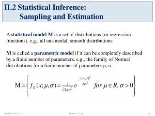
What’s New in This Chapter? • Usually population means (μ) are unknown and have to be estimated • To estimate μ, get a sample and find the sample mean, X • X estimates μ This is a parameter since it describes the population This is a statistic since it is derived from a sample
Estimating the Population Mean • This chapter discusses how good (reliable) this estimate is • The first two sections in this chapter pretend that the population mean (μ) is known • We do this to get some idea how the sample mean, X, “behaves”
How Does the Sample Mean Behave? • Suppose we were to get sample after sample, finding the sample mean each time • If we put these sample means into Excel and told it to make a histogram, what would it look like • In particular, does the histogram have a bell-shaped (normal) appearance?
Example 8.2 • Remember: For the first two sections, we’re pretending we know the population mean, μ • In this example, we’re interested in X = lifetime of a high-intensity light bulb • This example contains 20 samples of n = 10 bulbs each • Each sample is assumed to come from the population shown on the next slide
X μ = 400 The Population Shape for X = Lifetime of Bulb σ is 50 hours 250 300 350 450 500 550 Bulb lifetimes (in hours) are in here
20 Samples: X = Lifetime of Bulb Columns Q, R, S, T contain the last four samples Column V contains the 20 sample means followed by a summary of these means Column W contains the 20 sample standard deviations Notice The sample means are hanging around 400 The sample standard deviations are hanging around 50
The Main Thing The sample means don’t jump around as much (they have less variation) as the individual values Look at the variation in any of the samples in columns Q, R, S, and T Observe how much more variation there is in these four samples as compared to the sample means in column V This is much less than 50
X = Ht. 5.75’ X = Male Height This is picture #1: the shape of the population .25’ .25’ 5’ 5.25’ 5.5’ 6’ 6.25’ 6.5’ Nearly all heights are in here
X 5.75’ Looking at the Sample Means: Picture #2 This is the curve describing the average of n = 100 heights (measurements) This is a skinny normal curve 5.675’ 5.7’ 5.725’ 5.775’ 5.8’ 5.825’ Nearly all sample means are in here
A Whole Lot of Heights • The spreadsheet shown on the next two slides contains 50 samples of male heights • Each sample contains 100 heights • These are not actual heights but were computer generated • Each sample was selected from a normal population with a mean of 5.75’ and a standard deviation of .25’
The First 5 Samples of Heights The first 12 rows The last 5 rows
The Last 5 Samples of Heights The first 12 rows The last 5 rows
First Question • What proportion of male heights is > 5.8’? • This uses picture #1 since we’re talking about individual heights • This is a Chapter 7 problem (nothing new here) • P(X > 5.8’) =
X = Ht. 5.75’ X = Male Height Picture #1 This area 5’ 5.25’ 5.5’ 6’ 6.25’ 6.5’ 5.8’
P(Z > .2) This area is .5 - .0793 = .4207 This is also P(X > 5.8’) This area is .0793 Z -3 -2 -1 0 1 2 3 Z = .2
Second Question • What are the chances that an average of 100 heights is > 5.8’? • This type of question uses picture #2 • This is still an application of Chapter 7 but you need to use picture #2 and not picture #1 • You are trying to determine P( X > 5.8’) where X is the average of 100 heights
The Second Question • In picture #2, the mean of the normal curve is 5.75’ • This is the same as the mean of the population in picture #1 • The standard deviation of the normal curve in picture #2 is .025 • This is the population standard deviation in picture #1 divided by the square root of the sample size • Using picture #2,
X 5.75’ Picture #2 This is the curve describing the average of n = 100 heights .025 The skinny normal curve Need to find this area 5.675’ 5.7’ 5.725’ 5.775’ 5.8’ 5.825’
P(Z > 2) This area is .4772 This area is .5 - .4772 = .0228 Z -3 -2 -1 0 1 2 3 Z = 2
A Surprising Answer • Question: What happens to picture #2 if picture #1 is not a normal curve? • You might think that there is no answer here • Not true • The answer is that picture #2 is still a skinny normal curve (approximately) provided the sample size is “large” • Generally, n ≥ 30 is large enough
The Central Limit Theorem (CLT) • This is one of the biggest (maybe the biggest) results in statistics • It’s called the Central Limit Theorem (CLT) • It states that picture #2 is a (skinny) normal curve if the sample size is large (n ≥ 30) • In this case, it doesn’t matter what the shape of the population is (picture #1) • This will be illustrated in the next three slides
= 50 hours Population X µ = 400 hours 50 50 50 20 50 10 X X 400 (n = 20) 400 (n = 10) 50 100 X X 400 (n = 50) 400 (n = 100) Distribution of X This is picture #1 representing the lifetime of a light bulb (discussed in Chapter 7) Each of these is picture #2 = 11.18 = 15.81 = 7.07 = 5 Figure 8.6
Uniform population X 50 150 µ = 100 X X X (n = 5) (n = 2) (n = 30) Central Limit Theorem This is picture #1 The skinny normal curve Each of these is a picture #2 for different sample sizes Figure 8.10
Exponential population X X X X (n = 5) (n = 2) (n = 30) Central Limit Theorem This is picture #1 The skinny normal curve Each of these is a picture #2 for different sample sizes Figure 8.11
U-shaped population | µ X X | | | X X (n = 2) (n = 5) (n = 30) Central Limit Theorem This is picture #1 The skinny normal curve Each of these is a picture #2 for different sample sizes Figure 8.12
Recap of the CLT • Picture #1 describes the shape of the population of individual measurements • Maybe it’s normal, maybe it’s not • The CLT talks about picture #2 which describes the shape of the sample mean, X
X Recap of CLT This is normal provided ∙ n is large, or ∙ you have reason to believe picture #1 (the population) is normal This is called the standarderror of X A skinny normal curve
Section 8.3 • From now on, the population mean (μ) is unknown • The procedure is to get a sample from this population and find the sample mean, X • This will be illustrated in the next two slides using X = male height
X = Ht. μ = ? Estimating the Population Mean σ is known to be .25’ (3”) Picture #1 This is a parameter and it is unknown
Estimating the Population Mean • Get a sample of say, n = 100 heights • Suppose it turns out X = 5.77’ • What is μ (the average of all heights)? • We don’t know • But its estimate is X = 5.77’ • X is a statistic since it was derived from the sample
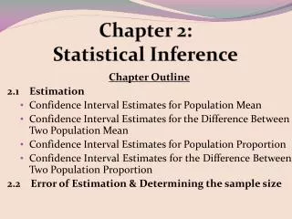
Estimating the Population Mean • Want to know: How good (reliable, precise) is this estimate? • We will answer this by providing a confidence interval for μ • We will end up saying something like - We are 95% confident that μ lies between 5.72’ and 5.82’ • 95% is called the confidence level and you can pick it
Estimating the Population Mean • Sample results: n = 100, X = 5.77’ • Notice that X = 5.77’ is in the middle of this confidence interval (5.72’ to 5.82’) • It always is • Rule: The narrower this interval is, the more reliable (precise) your estimate is
How to Find 5.72’ and 5.82’ • Provided (1) n is large or (2) you have reason to believe that picture #1 (the population) is believed to be normal, then mean = μ X is normal with standard deviation =
How to Find 5.72’ and 5.82’ • As a result, is a Z (you’ve standardized X) • Suppose we want a 95% confidence interval for the population mean, μ • You begin by working a backwards Z problem, illustrated on the next slide
How to Find 5.72’ and 5.82’ This area is half of .95 This is .475 This area is .95 Z -3 -2 -1 0 1 2 3 Z = -1.96 Z = 1.96
How to Find 5.72’ and 5.82’ • Using the previous Z curve, the following is true • P(-1.96 < Z < 1.96) is .95 • As a result, is .95 • After re-arranging, you get is .95
A 95% Confidence Interval for μ • A 95% confidence interval for μ is to • In our example, we’re assuming σ is .25’ • Sample results: n = 100 and x = 5.77’ • The resulting 95% confidence interval is shown on the next slide
A 95% Confidence Interval for μ • 5.77’ - 1.96 to 5.77’ + 1.96 • 5.77’ – 1.96(.025’) to 5.77’ + 1.96(.025’) • 5.77’ - .049’ to 5.77’ + .049’ • 5.72’ to 5.82’
Interpreting the Confidence Interval • We are 95% confident that the average of all heights (μ) is between 5.72’ and 5.82’ • We are 95% confident that the estimate of μ (namely, x = 5.77’) is within ± .049’ of the actual value of μ What we added and subtracted to/from 5.77’ to get the interval
Finding a 90% Confidence Interval This area is half of .9 This is .45 This area is .90 Z -3 -2 -1 0 1 2 3
Finding a 90% Confidence Interval • .45 is midway between .4495 and .4505 • .4495 belongs to 1.64 and .4505 belongs to 1.65 • We’ll use Z = 1.645 • Replace 1.96 with 1.645 in the previous • confidence interval
A 90% Confidence Interval for μ • 5.77’ - 1.645 to 5.77’ + 1.645 • 5.77’ – 1.645(.025’) to 5.77’ + 1.645(.025’) • 5.77’ - .041’ to 5.77’ + .041’ • 5.73’ to 5.81’ We are 90% confident that the estimate of μ (namely, x = 5.77’) is within ± .041’ of the actual value of μ
Using the Excel Macro • You begin by entering the sample values in column A • The macro will be illustrated using a sample of 100 heights in column A • The population standard deviation is known to be .25 • The “Population mean (Z statistic)” macro should be selected
Using the Excel Macro Enter: 1 for a 99% confidence interval 5 for a 95% confidence interval 10 for a 90% confidence interval etc.
Macro Output Agrees with the previous results
X = Ht. Section 8.4 – σ is Unknown σ = ? Picture #1 must be normal for this situation μ = ?
Section 8.4 – σ is Unknown • Sample results: n = 15 (a small sample) X = 5.72’ s = .31’ Estimates μ These are statistics Estimates σ μ and σ are parameters