Download
1 / 40
420 likes | 788 Vues
Point and Confidence Interval Estimation of a Population Proportion, p. We are frequently interested in estimating the proportion of a population with a characteristic of interest, such as: the proportion of smokers the proportion of cancer patients who survive at least 5 years

E N D
Point and Confidence Interval Estimation of a Population Proportion, p
We are frequently interested in estimating the proportion of a population with a characteristic of interest, such as: • the proportion of smokers • the proportion of cancer patients who survive at least 5 years • the proportion of new HIV patients who are female
If we take a random sample from a population • observe the number of subjects with the characteristic of interest (# of “successes”) • we are observing a binomial random variable. • Now, however, we will focus on • estimating the true proportion , p, in the population • rather than focusing on the count.
Again, one way to deal with this type of data is to define a random variable X that can take two values: • X = 1, if characteristic is present – a “success” • X = 0, if characteristic is absent – a “failure” • Then • if we sum all values in a population, • we are summing zeros and ones – • this will give a count of the number of individuals in the population with the characteristic:
The population mean is the Proportion of individuals in population with the characteristic: The sample proportion is then: Therefore, p is the estimator of p, the proportion with a characteristic of interest.
By the Central Limit Theorem, we know, for n large even when X is not normally distributed. When X is a 0,1 variable, for n large we know from the central limit theorem.
What is the variance, s2, for a 0,1 variable? We know By use of algebra, and the fact that xs2 = xs. for a 0,1 variable, we can show that
For those who want the algebra: expand x2 = x, for 0,1 sum over constant
Hence, The standard error of the sample proportion is Standard error of P:
We also know, by the central limit theorem, that for large n, P is approximately normally distributed: For Estimation of the population proportion, p: Point Estimate:Confidence Interval Estimate:
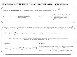
Example: Suppose that a sample of 1000 voters is taken to determine presidential preference. In this sample, 585 persons indicated that they would vote for candidate A. Construct a 95% confidence interval estimate for the true proportion, p, in the population planning to vote for candidate A. The confidence interval forptakes the form:
The point estimate of the proportion is: p= (585/1000) = .585 • The 95% confidence interval estimator of p is • However we don’t know p, so we will use p in it’s place to estimate the standard error:
The 95% CI on the proportion preferring Candidate A is (.554, .616). This does not include the value .50: Either we obtained an unusually large sample mean (such that the interval estimate did not overlap µ=0.5) if µ really is .5, or the population mean is not .5, suggesting that candidate A will win the election.
When is the sample large enough to use the normal approximation to the binomial? • When (n)(π)5, and (n)(1-π)5 • That is, • when both the expected number of successesand the expected number of failures is greater than 5.
Aside: improve to the normal Appoximation for a Binomial • The Binomial distribution is discrete, while the normal distribution is continuous. When the true proportion,π, is known, we can match the binomial distribution better to a normal distribution by including a correction. The correction is called the ‘continuity correction’. • For example, when π = .5, and n = 10, to approximate We use instead the normal approximation for the probability
Example of ‘Continuity Correction' to the Normal Approximation to the Binomial. Suppose π = .5 and n = 16. Compare the exact normal approximation and continuity corrected values of P(.4375 ≤ P ≤ .5). • From Binomial Table: • Using Normal Approximation, no correction • Using Correction:
Using P in place of p to estimate the standard errorsp: • 1.If (n)(π)5 and (n)(1-π)5, use P: • 2.Otherwise, a) Assume π=.5,or b) use an ‘exact ’method for the CI • We do this to avoid underestimating the variance, p(1– p) which is at a maximum when p=.5 • Don’t use Student’s t with proportions since the assumption of normality of the underlying population elements is not satisfied by a 0,1 variable.
What do we use when the normal approximation is not appropriate? • Exact Binomial Confidence Intervals for p can be computed: • Solve for x in the following and then substitute into p= x/n: • Lower Limit: • Upper Limit: • Clearly, exact binomial CI is not simple to compute
Go to Minitab or other software Stat Basic Statistics 1 Proportion Leave blank for Binomial CI; Check for Normal approx. n x
EXACT Binomial: Test and CI for One Proportion Test of p = 0.5 vs p not = 0.5 Exact Sample X N Sample p 95.0% CI P-Value 1 585 1000 0.585 (0.553748, 0.615750) 0.000 Normal Approximation: Test and CI for One Proportion Test of p = 0.5 vs p not = 0.5 Sample X N Sample p 95.0% CI Z-Value P-Value 1 585 1000 0.585 (0.554461, 0.615539) 5.38 0.000
Sample Size Estimation when the goal is Estimating a Population Proportion, p • The pattern is the same as when goal is estimation of a mean: • If we know • the desired precision (width of interval) • confidence level • “guess” of the proportion to get std error • we can estimate the sample size, n.
The width of a confidence interval for P is: w = 2[z1-a/2 (sP)] , where sP is the standard error of P w ) ( P P – z1-a/2(sP) P + z1-a/2(sP) Using we have
Solving for n gives us • Note: • this requires information about p, which is our goal! • However, p(1–p) is at a maximum when p=.5 • To be conservative • (over- rather than under-estimate sample size) • use (.5) in place of p
Substituting in .5 for p gives a conservative sample size estimator of:
Example: • For an election poll, how many voters should be surveyed to estimate the proportion, to within 5%, in favor of re-electing the current mayor, with 95% confidence? • We have a confidence level, 1–a = .95 z.975 = 1.96 • We have a desired width of 5% = .05, w = .10 • Conservative: n = (z1-a/2)2/w2 = (1.96)2/(.10)2 = 384.16 • We should poll 385 voters to achieve a 95% CI of 5%
What if we have some information on p? • A previous poll tells us that the current office-holder had ~ 75% of the voter support. • Assuming p = .75: • n = 4p(1–p)(z1-a/2)2/w2 • = 4(.75)(.25)(1.96)2/(.10)2 = 288.12 • Using available information • we get a sample size estimate of 289 voters • which can save us considerable time and expense, compared to the more conservative estimate.
Confidence Interval Calculation for the Difference between two proportions, p1 – p2, Two independent groups • We are often interested in comparing proportions from 2 populations: • Is the incidence of disease A the same in two populations? • Patients are treated with either drug D, or with placebo. Is the proportion “improved” the same in both groups?
Suppose we take independent, random samples from two groups, and estimate a proportion in each. For large enough sample size, we know: Then the standard error of the difference between the sample proportions is the square root of the sum of the variances:
Or, since we don’t know the true proportions, the sample estimate of the standard error: Thus, for n large, the (1-a) confidence interval estimator is:
Example: In a clinical trial for a new drug to treat hypertension, 50 patients were randomly assigned to receive the new drug, and 50 patients to receive a placebo. 34 of the patients receiving the drug showed improvement, while 15 of those receiving placebo showed improvement. Compute a 95% confidence interval estimate for the difference between proportions improved.
Point Estimate of (p1 – p2): • p1 = 34/50 = .68 • p2 = 15/50 = .30 (p1 – p2)= .68 – .30 = .38 • Since we have n1 = n2 = 50, our sample size is large enough to use the sample estimate of standard error:
Confidence coefficient: For 1 – a = .95, z1-a/2 = z.975 = 1.96 • Confidence Interval Estimate: • The 95% CI estimate is: • (.199 , .561) or (19.9% , 56.1%) • The difference between proportions improved is bounded away from zero – it seems that the proportion improved by the drug is clearly greater than the proportion by placebo.
Using Minitab: Stat Basic Statistics 2 Proportions Enter sample sizes n1 and n2 Enter # of successes x1 and x2
Test and Confidence Interval for Two Proportions Sample X N Sample p 1 34 50 0.680000 2 15 50 0.300000 Estimate for p(1) - p(2): 0.38 95% CI for p(1) - p(2): (0.198748, 0.561252)
The same cautions apply here, as for estimates for a single proportion • the sample size should be large enough in each group, so that the normal approximation will hold: • nπ5 and n(1-π)5 for each sample • Otherwise: a) use .5 in place of π when estimating the variance for the confidence interval.b) use some other method. • Minitab offers the option to compute a pooled estimate of the standard error
And in summary: • Confidence interval estimates provide • a range of likely values • an associated probability, or confidence level. • The width of the confidence interval depends upon: • The underlying variability in the population • The sample size • The confidence level
It is important to keep track of assumptions that we must make about the data: • Samples should be selected randomly • selection of any element is independent of selection of any others • For many cases, we must assume that the underlying population follows a normal distribution • without this assumption, probabilities computed using the • t-distribution • c2–distribution • F-distribution may not be correct.
When we speak of “knowing” the population variance, s2, • we really mean that we have an outside source of information • previous research, census data, etc. • the key is that we are not using the sample estimate, s2, based upon the current sample.
The key to confidence interval estimation is to know • what parameter you are estimating • the point estimate of the parameter • the confidence level • what distributional assumptions are required • the associated distribution for computing probabilities. • I have started a summary table for you below – completing this table will be a good review exercise.