Chapter 8 Hypothesis Testing
Chapter 8 Hypothesis Testing. 8-1 Review and Preview 8-2 Basics of Hypothesis Testing 8-3 Testing a Claim about a Proportion 8-4 Testing a Claim About a Mean: Known 8-5 Testing a Claim About a Mean: Not Known 8-6 Testing a Claim About a Standard Deviation or Variance.

Chapter 8 Hypothesis Testing
E N D
Presentation Transcript
Chapter 8Hypothesis Testing 8-1 Review and Preview 8-2 Basics of Hypothesis Testing 8-3 Testing a Claim about a Proportion 8-4 Testing a Claim About a Mean: Known 8-5 Testing a Claim About a Mean: NotKnown 8-6 Testing a Claim About a Standard Deviation or Variance
In statistics, a hypothesis is a claim or statement about a property of a population. A hypothesis test (or test of significance) is a standard procedure for testing a claim about a property of a population. Definitions
The main objective of this chapter is to develop the ability to conduct hypothesis tests for claims made about population parameter ( population proportion , a population mean , or a population standard deviation ) Main Objective
When conducting hypothesis tests as before jumping directly to procedures and calculations, be sure to consider the context of the data, the source of the data, and the sampling method used to obtain the sample data. Caution
8.2 Basics of Hypothesis Testing
The null hypothesis and alternative hypothesis from a given claim • The value of the test statistic, given a claim and sample data • Critical value(s), given a significance level • P-value, given a value of the test statistic • The conclusion about a claim in simple and nontechnical terms
Rare Event Rule for Inferential Statistics If, under a given assumption, the probability of a particular observed event is exceptionally small, we conclude that the assumption is probably not correct.
Alternative Hypothesis: The alternative hypothesis (denoted by ) is the claim or research hypothesis we wish to establish. The symbolic form of the alternative hypothesis must use one of these symbols: .
Null Hypothesis: The null hypothesis (denoted by ) is a statement that nullifies the research hypothesis We test the null hypothesis directly. Either reject or fail to reject .
Test Statistic The test statistic is a value used in making a decision about the null hypothesis, and is found by converting the sample statistic to a score with the assumption that the null hypothesis is true.
Test Statistic - Formulas Test statistic for proportion Test statistic for mean Test statistic for standard deviation
example • claim that the XSORT method of gender selection increases the likelihood of having a baby girl. • Preliminary results from a test of the XSORT method of gender selection involved 14 couples who gave birth to 13 girls and 1 boy.
Example: We know from previous chapters that a z score of 3.21 is “unusual” (because it is greater than 2). It appears that in addition to being greater than 0.5, the sample proportion of 13/14 or 0.929 is significantly greater than 0.5. The figure on the next slide shows that the sample proportion of 0.929 does fall within the range of values considered to be significant because
Example: Sample proportion of: or Test Statistic z = 3.21 they are so far above 0.5 that they are not likely to occur by chance (assuming that the population proportion is p = 0.5).
Critical Region The critical region (or rejection region) is the set of all values of the test statistic that cause us to reject the null hypothesis. For example, see the red-shaded region in the previous figure.
Significance Level The significance level (denoted by) is the probability that the test statistic will fall in the critical region when the null hypothesisis actually true. This is the sameintroduced in Section 7-2. Commonchoices forare 0.05, 0.01, and 0.10.
Critical Value A critical value is any value that separates the critical region (where we reject the null hypothesis) from the values of the test statistic that do not lead to rejection of the null hypothesis. The critical values depend on the nature of the null hypothesis, the sampling distributionthat applies, andthe significance level. See the previous figure where the critical value ofz= 1.645corresponds to a significance level of .
P-Value The P-value (or p-value or probabilityvalue) is the probability of getting a value of the test statistic that is at least as extreme as the one representing the sample data, assuming that the null hypothesis is true. Critical region in the left tail: P-value = area to the left of the test statistic Critical region in the right tail: P-value = area to the right of the test statistic Critical region in two tails: P-value = twice the area in the tail beyond the test statistic
P-Value The null hypothesis is rejected if the P-value is very small, such as 0.05 or less. Here is a memory tool useful for interpreting the P-value: If the P is low, the null must go. If the P is high, the null will fly.
Procedure for Finding P-Values Figure 8-5
Example Consider the claim that with the XSORT method of gender selection, the likelihood of having a baby girl is different from p = 0.5, and use the test statistic z = 3.21 found from 13 girls in 14 births. First determine whether the given conditions result in a critical region in the right tail, left tail, or two tails, then use Figure 8-5 to find the P-value. Interpret the P-value.
Example Ho: Ha: The critical region is in two tails find the P-value for a two-tailed test, the P-value is twice the area to the right of the test statistic z = 3.21. Use Z-Table to find that the area to the right of z = 3.21 is 0.0007. In this case, the P-value is twice the area to the right of the test statistic, so we have:P-value = 2 0.0007 = 0.0014
Example The P-value is 0.0014. The small P-value of 0.0014 shows that there is a very small chance of getting the sample results that led to a test statistic of z = 3.21. This suggests that with the XSORT method of gender selection, the likelihood of having a baby girl is different from 0.5.
Types of Hypothesis Tests:Two-tailed, Left-tailed, Right-tailed The tails in a distribution are the extreme regions bounded by critical values. Determinations of P-values and critical values are affected by whether a critical region is in two tails, the left tail, or the right tail. It therefore becomes important to correctly characterize a hypothesis test as two-tailed, left-tailed, or right-tailed.
Two-tailed Test Means less than or greater than is divided equally between the two tails of the critical region
Left-tailed Test Points Left the left tail
Right-tailed Test Points Right
Conclusions in Hypothesis Testing We always test the null hypothesis. The initial conclusion will always be one of the following: 1. Rejectthe null hypothesis. 2. Fail to reject the null hypothesis.
Decision Criterion P-value method: Using the significance level : If P-value ,reject. If P-value , fail to reject .
Decision Criterion Traditional method: If the test statistic falls within the critical region, reject. If the test statistic does not fall within the critical region, fail to reject .
Decision Criterion Another option: Instead of using a significance level such as 0.05, simply identify theP-value and leave the decision to the reader.
Decision Criterion Confidence Intervals A confidence interval estimate of a population parameter contains the likely values of that parameter. We should therefore reject a claim that the population parameter has a value that is not included in the confidence interval.
Caution In some cases, a conclusion based on a confidence interval may be different from a conclusion based on a hypothesis test.
Wording of Final Conclusion Figure 8-7
Caution Never conclude a hypothesis test with a statement of “reject the null hypothesis” or “fail to reject the null hypothesis.” Always make sense of the conclusion with a statement that uses simple nontechnical wording that addresses the original claim.
Accept Versus Fail to Reject Some texts use “accept the null hypothesis.” We are not proving the null hypothesis. Fail to rejectsays more correctly The available evidence is not strong enough to warrant rejection of the null hypothesis (such as not enough evidence to convict a suspect).
Type I Error A Type I error is the mistake of rejecting the null hypothesis when it is actually true. The symbol (alpha) is used to represent the probability of a type I error.
Type II Error A Type II error is the mistake of failing to reject the null hypothesis when it is actually false. The symbol(beta) is used to represent the probability of a type II error.
Example: Assume that we are conducting a hypothesis test of the claim that a method of gender selection increases the likelihood of a baby girl, so that the probability of a baby girls is . Here are the null and alternative hypotheses: , and . a) Identify a type I error. b) Identify a type II error.
Example: a) A type I error is the mistake of rejecting a true null hypothesis, so this is a type I error: Conclude that there is sufficient evidence to support , when in reality . b) A type II error is the mistake of failing to reject the null hypothesis when it is false, so this is a type II error: Fail to reject (and therefore fail to support ) when in reality .
Controlling Type I and Type II Errors For any fixed , an increase in the sample size nwill cause a decrease in For any fixed sample size n, a decrease in will cause an increase in . Conversely, an increase in will cause a decrease in . To decrease both and , increase the sample size.
Part 2: Beyond the Basics of Hypothesis Testing: The Power of a Test
Definition The powerof a hypothesis test is the probability of rejecting a false null hypothesis. The value of the power is computed by using a particular significance level and a particular value of the population parameter that is an alternative to the value assumed true in the null hypothesis. That is, the power of the hypothesis test is the probability of supporting an alternative hypothesis that is true.
Power and theDesign of Experiments Just as 0.05 is a common choice for a significance level, a power of at least 0.80 is a common requirement for determining that a hypothesis test is effective.
Recap • In this section we have discussed: • Null and alternative hypotheses. • Test statistics. • Significance levels. • P-values. • Decision criteria. • Type I and II errors. • Power of a hypothesis test.
8.3 Testing a claim about a Proportion
Notation = population proportion (used in the null hypothesis) = number of trials (sample proportion)