Download
1 / 30
300 likes | 577 Vues
Chapter 8 Introduction to Hypothesis Testing. Chapter Goals. After completing this chapter, you should be able to: Formulate null and alternative hypotheses for applications involving a single population mean Formulate a decision rule for testing a hypothesis

E N D
Chapter 8Introduction to Hypothesis Testing Fall 2006 – Fundamentals of Business Statistics
Chapter Goals After completing this chapter, you should be able to: • Formulate null and alternative hypotheses for applications involving a single population mean • Formulate a decision rule for testing a hypothesis • Know how to use the test statistic, critical value, and p-value approaches to test the null hypothesis Fall 2006 – Fundamentals of Business Statistics
Testing Theories Hypotheses Competing theories that we want to test about a population are called Hypotheses in statistics. Specifically, we label these competing theories as Null Hypothesis (H0) and Alternative Hypothesis (H1 or HA). H0 : The null hypothesis is the status quo or the prevailing viewpoint. HA : The alternative hypothesis is the competing belief. It is the statement that the researcher is hoping to prove. Fall 2006 – Fundamentals of Business Statistics
The Null Hypothesis, H0 • Begin with the assumption that the null hypothesis is true • Refers to the status quo • Always contains “=” , “≤” or “” sign • May or may not be rejected (continued) Fall 2006 – Fundamentals of Business Statistics
The Alternative Hypothesis, HA • Challenges the status quo • Never contains the “=” , “≤” or “” sign • Is generally the hypothesis that is believed (or needs to be supported) by the researcher • Provides the “direction of extreme” Fall 2006 – Fundamentals of Business Statistics
Hypothesis Testing Process Claim:the population mean age is 50. (Null Hypothesis: Population H0: = 50 ) Now select a random sample x = likely if = 50? Is 20 Suppose the sample If not likely, REJECT mean age is 20: x = 20 Sample Null Hypothesis Fall 2006 – Fundamentals of Business Statistics
Deciding Which Theory to Support Decision making is based on the “rare event” concept. Since the null hypothesis is the status quo, we assume that it is true unless the observed result is extremely unlikely (rare) under the null hypothesis. • Definition: If the data were indeed unlikely to be observed under the assumption that H0is true, and therefore we reject H0in favor of HA, then we say that the data are statistically significant. Fall 2006 – Fundamentals of Business Statistics
Reason for Rejecting H0 Sampling Distribution of x x = 50 If H0 is true Fall 2006 – Fundamentals of Business Statistics
Level of Significance, • Defines unlikely values of sample statistic if null hypothesis is true • Defines rejection region of the sampling distribution • Is designated by , (level of significance) • Is selected by the researcher at the beginning • Provides the critical value(s) of the test Fall 2006 – Fundamentals of Business Statistics
Level of Significance and the Rejection Region a Level of significance = Represents critical value H0: μ≥ 3 HA: μ < 3 a Rejection region is shaded 0 Lower tail test H0: μ≤ 3 HA: μ > 3 a 0 Upper tail test H0: μ = 3 HA: μ≠ 3 a a /2 /2 Two tailed test 0 Fall 2006 – Fundamentals of Business Statistics
Critical Value Approach to Testing • Convert sample statistic (e.g.: ) to test statistic ( Z* or t* statistic ) • Determine the critical value(s) for a specifiedlevel of significance from a table or computer • If the test statistic falls in the rejection region, reject H0 ; otherwise do not reject H0 Fall 2006 – Fundamentals of Business Statistics
x Critical Value Approach to Testing • Convert sample statistic ( ) to a test statistic ( Z* or t* statistic ) Sample Size? Is X ~ N? Yes No Small Large (n ≥ 100) Is s known? Yes No, use sample standard deviation s 2. Use T~t(n-1) 1. Use Z~N(0,1)
Calculating the Test Statistic: Z • Two-Sided: H0: μ = μ0; HA: μ ≠ μ0 • Reject H0if Z* > Z(0.5−α/2) or Z* < −Z(0.5−α/2), otherwise do not reject H0 • One-Sided Upper Tail: H0: μ ≤ μ0; HA: μ >μ0 • Reject H0if Z* > Z(0.5−α), otherwise do not reject H0 • One-Sided Lower Tail: H0: μ ≥ μ0; HA: μ <μ0 • Reject H0if Z* < -Z(0.5−α), otherwise do not reject H0 Fall 2006 – Fundamentals of Business Statistics
Two-Sided: H0: μ = μ0; HA: μ ≠ μ0 • Reject H0if , otherwise do not reject H0 • One-Sided Upper Tail: H0: μ ≤ μ0; HA: μ >μ0 • Reject H0if , otherwise do not reject H0 • One-Sided Lower Tail: H0: μ ≥ μ0; HA: μ <μ0 • Reject H0if , otherwise do not reject H0 T test Statistic Fall 2006 – Fundamentals of Business Statistics
Review: Steps in Hypothesis Testing • Specify the population value of interest • Formulate the appropriate null and alternative hypotheses • Specify the desired level of significance • Determine the rejection region • Obtain sample evidence and compute the test statistic • Reach a decision and interpret the result Fall 2006 – Fundamentals of Business Statistics
Hypothesis Testing Example Test the claim that the true mean # of TV sets in US homes is less than 3. Assume that s = 0.8 • Specify the population value of interest • Formulate the appropriate null and alternative hypotheses • Specify the desired level of significance
Hypothesis Testing Example • 4. Determine the rejection region (continued) = Reject H0 Do not reject H0 0 Reject H0 if Z* test statistic < otherwise do not reject H0 Fall 2006 – Fundamentals of Business Statistics
Hypothesis Testing Example • 5. Obtain sample evidence and compute the test statistic A sample is taken with the following results: n = 100, x = 2.84( = 0.8 is assumed known) • Then the test statistic is: Fall 2006 – Fundamentals of Business Statistics
Hypothesis Testing Example (continued) • 6. Reach a decision and interpret the result = z Reject H0 Do not reject H0 0 Since Z* = -2.0 < , Fall 2006 – Fundamentals of Business Statistics
p-Value Approach to Testing • p-value: Probability of obtaining a test statistic more extreme than the observed sample value given H0 is true • Also called observed level of significance • Smallest value of for which H0 can be rejected Fall 2006 – Fundamentals of Business Statistics
p-Value Approach to Testing • Convert Sample Statistic to Test Statistic ( Z* or t* statistic ) • Obtain the p-value from a table or computer • Compare the p-value with • If p-value < , reject H0 • If p-value , do not reject H0 Fall 2006 – Fundamentals of Business Statistics
P-Value Calculation Z test statistic • Two-Sided: 2 ×min {P(Z ≥ Z*,Z ≤ Z*)} • One-Sided Upper Tail P(Z ≥ Z*) • One-Sided Lower Tail P(Z ≤ Z*) T test statistic • Two-Sided: 2 ×min {P(t ≥ t*,t ≤ t*)} • One-Sided Upper Tail P(t ≥ t*) • One-Sided Lower Tail P(t ≤ t*) Fall 2006 – Fundamentals of Business Statistics
p-value example Fall 2006 – Fundamentals of Business Statistics
Example: Upper Tail z Test for Mean ( Known) A phone industry manager thinks that customer monthly cell phone bill have increased, and now average over $52 per month. The company wishes to test this claim. (Assume = 10 is known) Form hypothesis test: H0: μ≤ 52 the average is not over $52 per month HA: μ > 52 the average is greater than $52 per month (i.e., sufficient evidence exists to support the manager’s claim) Fall 2006 – Fundamentals of Business Statistics
Example: Find Rejection Region (continued) Reject H0 = Do not reject H0 Reject H0 0 Fall 2006 – Fundamentals of Business Statistics
Example: Test Statistic Obtain sample evidence and compute the test statistic A sample is taken with the following results: n = 64, x = 53.1 (=10 was assumed known) • Then the test statistic is: (continued) Fall 2006 – Fundamentals of Business Statistics
Example: Decision (continued) Reach a decision and interpret the result: Reject H0 = Do not reject H0 Reject H0 0 Fall 2006 – Fundamentals of Business Statistics
p -Value Solution Calculate the p-value and compare to (continued) 0 Do not reject H0 Reject H0 Fall 2006 – Fundamentals of Business Statistics
The average cost of a hotel room in New York is said to be $168 per night. A random sample of 25 hotels resulted in = $172.50 and s = $15.40. Test at the = 0.05 level. (Assume the population distribution is normal) Example: Two-Tail Test( Unknown) H0:μ= 168HA:μ ¹168 Fall 2006 – Fundamentals of Business Statistics
Outcomes and Probabilities Possible Hypothesis Test Outcomes State of Nature Decision H0 True H0 False Do Not No error (1 - ) Type II Error ( β ) Reject Key: Outcome (Probability) a H 0 Reject Type I Error ( ) No Error ( 1 - β ) H a 0 Fall 2006 – Fundamentals of Business Statistics