Introduction to Hypothesis Testing
Introduction to Hypothesis Testing. Chapter 11. Introduction . The purpose of hypothesis testing is to determine whether there is enough statistical evidence supporting a certain belief about a parameter. Examples


Introduction to Hypothesis Testing
E N D
Presentation Transcript
Introduction to Hypothesis Testing Chapter 11
Introduction • The purpose of hypothesis testing is to determine whether there is enough statistical evidence supporting a certain belief about a parameter. • Examples • Is there statistical evidence in a random sample of potential customers, that support the hypothesis that more than p% of all potential customers will purchase a new products? • Is the hypothesis that a certain drug is effective supported by the level of improvement in patients’ conditions after treated with the drug, compared with this of another group of patients who were given a placebo?
11.1 Concepts of Hypothesis Testing • Two hypotheses are defined. H0: The null hypothesis. Under this hypothesis we specify our current belief about the parameter we test. (m = 170, p = .4, etc.) H1: The alternative hypothesis. Under this hypothesis we specify a range of values for the parameter tested (m > 170; p ¹ .4; etc.) effected by some action taken. This is the hypothesis we try to prove!
Concepts of Hypothesis Testing • The two hypotheses are stated, and a test is run to determine whether a sample statistic supports the rejection of H0 in favor of H1. H0: m = 170 H1: m > 170
If we have little incentive to believe m > 170because and m are relatively close. The Concept of Hypothesis Testing Let’s assume H0 is true: m = 170 A sample is drawn.Assume the sample mean = 180. m = 170
If we have much more incentive to believe m > 170 because falls far above m. The Concept of Hypothesis Testing Let’s assume H0 is true: m = 170 A sample is drawn.Now assume the sample mean = 250. The question is: How far is far? Is 250 sufficiently larger than 170 for us to believe that m > 170? Click. m = 170
This is the probability that when m > 170 This is the probability that when m = 170 As you can see it becomes more likely that when m > 170 The Concept of Hypothesis Testing Let’s assume H0 is true: m = 170 You may want to think about it as follows. Click: With m = 170… click If m were greater than 170… click m = 170 m> 170
The Concept of Hypothesis Testing • We’ll look next at the probability thatas a tool to help decide whether we shouldreject H0. • This idea will be further discussed (with a somewhat more computational flavor) as example 1 is presented next. • Pay attention!
11.2 Testing the Population Mean when the Population Standard Deviation is Known • Example 1: Department Store new Billing System • A new billing system for a department store will be cost- effective only if the mean monthly account is more than $170. • A sample of 400 accounts has a mean of $178. • If the accounts are approximately normally distributed with s = $65, can we conclude that the new system will be cost effective? (can we conclude from the sample result that the accounts population mean is greater than 170?)
Testing the Population Mean (s is Known) • Example 1 - Solution • The population of interest is the credit accounts at the store. • We want to show that the mean account for all customers is greater than $170. This is what you want to prove H1 : m > 170 • The null hypothesis must specify the values of the parameter m, not included in H1 H0 : m£ 170
Testing the Population Mean (s is Known) • To better understand the hypotheses testing concept let us ask the following question: • If H0 is true (m = 170) how likely is it a sample of 400 accounts have a sample mean at least as large as 178? • Answer: By the central limit theorem • To illustrate, by sheer chance, out of 10000 samples of 400 accounts each only 69 samples will have a sample mean of 178 or more, if indeed m = 170. • It seems there must be another reason (rather than just “chance”) why the event has occurred. Click. • Most likely m > 170, which explains better why . That is, H0 should be rejected in favor of H1
Types of Errors • Testing the hypotheses, two types of errors may occur when deciding whether to reject H0 based on the sample result. • Type I error: Reject H0 when it is true. • Type II error: Do not reject H0 when it is false.
Types I and Type II Errors in Example 1 • Example 1 - continued • Type I error: Believe that m > 170 when the real value of m is 170 (reject H0 in favor of H1 when H0 is true). • Type II error: Believe that m£ 170 when the real value of m > 170 (do not reject H0 when it is false).
Critical value Controlling the probability of conducting a type I error • Recall: H0:m£ 170 H1: m > 170, Since the alternative hypothesis has the form of m > m0, H0 is rejected if is sufficiently large! Our job is to determine a critical value for the sample mean. H0 is rejected if the sample mean exceeds that critical value. m = 170 H0
Note. May exceed a critical value (leading to the rejection of H0) but the population mean may still be 170. We don’t want the probability of this event exceeds some acceptable value (a). Critical value Controlling the probability of conducting a type I error • Recall: H0:m£ 170 H1: m > 170, So how do we determine this critical value? We turn to a type I error and limit the probabilityit occurs. m = 170 H0
Approaches to Testing • There are two approaches to test whether the sample mean supports the alternative hypothesis (H1) • The rejection region method is mandatory for manual testing (but can be used when testing is supported by a statistical software) • The p-value method which is mostly used when a statistical software is available. • Both involve an upper limit we set on the probability of conducting a type I error.
The Rejection Region Method The null hypothesis is rejected in favor of the alternative hypothesis if a test statistic falls in the rejection region.
The Rejection Region Method of a Right Hand Tail Test • Example 1 – solution continued • Recall:H0: m £ 170 H1: m > 170. • Define a critical value for that is just large enough to reject the null hypothesis. • Reject the null hypothesis if
Determining the Critical Value for the Rejection Region of a Right Hand Tail Test • Allow the probability of committing a type I error be a (also called the significance level). • Find a critical value of the sample mean that is just large enough to guarantee that the actual probability of committing a type I error does not exceed a.
a Determining the Critical Value for a Right Hand Tail Test Example 1 – solution continued m = 170 P(commit a type I error) = P(reject H0 when H0 is true) From the central limit theorem:
a Determining the Critical Value for a Right Hand Tail Test Example 1 – solution continued m = 170 and
Simple algebra Determining the Critical Value for a Right Hand Tail Test Example 11.1 – solution continued a
Determining the Critical Value for a Right Hand Tail Test Conclusion Since the sample mean (178) is greater than the critical value of 175.34, there is sufficient evidence to infer that the mean monthly balance is greater than $170 at 5% significance level.
Determining the Critical Value for a Right Hand Tail Test Interpretation The null hypothesis is rejected in favor of the alternative hypothesis because the sample mean falls in the rejection region. Still we may be erroneous when rejecting the null hypothesis, since m could be 170, but the chance we make such a mistake is not greater than 5% (the significance level).
H0: m = m0 The standardized test statistic • Instead of using the statistic , we can use the standardized value z. • If the alternative hypothesis is: H1: m > m0, then the rejection region is
The standardized test statistic • Example 1 - continued • We redo this example using the standardized test statistic. Recall: H0: m= 170 H1: m > 170 • Test statistic: • Rejection region: z > z.05 = 1.645.
The standardized test statistic • Example 11.1 - continued • Conclusion • Since Z = 2.46 > 1.645, reject the null hypothesis in favor of the alternative hypothesis.
The P-value Method • Ask the question: How probable is it to obtain a sample mean at least as extreme as 178, if the population mean is 170 (H0 is true)?
P-value method The probability of observing a test statistic at least as extreme as 178, given that m = 170 is… The p-value
Note how the event is rare under H0 when but... …it becomes more probable under H1, when Interpreting the p-value Because the probability that the sample mean will assume a value of more than 178 when m = 170 is so small (.0069), there are reasons to believe that m > 170.
Interpreting the p-value We can conclude that the smaller the p-value the more statistical evidence exists to support the alternative hypothesis.
P-value – Summary • The p-value provides information about the amount of statistical evidence that supports the alternative hypothesis. • The p-value of a test is the probability of observing a test statistic at least as extreme as the one computed, given that the null hypothesis is true.
Interpreting the p-value • Describing the p-value • If the p-value is less than 1%, there is overwhelming evidence that supports the alternative hypothesis. • If the p-value is between 1% and 5%, there is a strong evidence that supports the alternative hypothesis. • If the p-value is between 5% and 10% there is a weak evidence that supports the alternative hypothesis. • If the p-value exceeds 10%, there is no evidence that supports the alternative hypothesis.
a = 0.05 The p-value and the rejection region methods • The p-value can be used when making decisions based on rejection region methods as follows: • Compare the p-value to a. Reject the null hypothesis only if the p value < a; Otherwise, do not reject the null hypothesis. Note: 0.0069 < 0.05! The p-value = 0.0069
Reject H0 if falls here Left Hand Tail Test H0: m =m0H1: m < m0 Critical value
An Example for a Left Hand Tail Test • The SSA envelop plan example. • The chief financial officer in FedEx believes that including a stamped self-addressed (SSA) envelop in the monthly invoice sent to customers will decrease the amount of time it take for customers to pay their monthly bills. • Currently, customers return their payments in 22 days on the average, with a standard deviation of 6 days.
An Example for a Left Hand Tail Test • The SSA envelop example – continued • A random sample of 220 customers was selected and SSA envelops were included with their invoice packs. • The time it took customers to pay their bill was recorded (see SSA) • Can the CFO conclude that the plan will be successful at 10% significance level?
An Example for a Left Hand Tail Test • The SSA envelop example – Solution • The parameter tested is the ‘population mean of the payment time’ (m). • Since the CFO wants to prove that the plan will be successful, we test whether H1: m < 22 • Accordingly, The null hypothesis is: H0: m= 22
Rejection Region m=22 An Example for a Left Hand Tail Test • The SSA envelop example – Solution continued • The rejection region: It makes sense to believe that m < 22 if the sample mean is sufficiently smaller than 22. • Thus, reject the null hypothesis if
-za 0 a The Standardized Rejection Region for a Left Hand Tail Test • Note that a is small (certainly less than 50%). So the critical Z value must be negative. Click. The standardized rejection region is:
This is the sample mean -za 0 An Example for a Left Hand Tail Test • The SSA envelop example – Solution continued • The standardized approach: From the data we find that the sample mean = 21.44 • Za = Z.10 = 1.285 so,-Z.10 = -1.285 • Conclusion: Since -1.384 < –1.285 reject the null hypothesis.
The p – value approach for a Left Hand Tail Test • The SSA envelop example – Solution continue The p value = P(Z<-1.384) = .0831 and a = 0.1 Since .0831 < .1 (p value<a) reject the null hypothesis. pvalue -1.384 -1.285
Reject H0 if falls here Reject H0 if falls here Critical value Critical value An Example for a Two Tail Test H0: m=m0 H1: m¹ m0
An Example for a Two Tail Test • Example 2 • AT&T has been challenged by competitors whose rates arguably resulted in lower bills. • A statistician believes the monthly mean and standard deviation of the long-distance bills for all AT&T residential customers are $17.85 and $3.87 respectively.
An Example for a Two Tail Test • Example 2 - continued • A random sample of 25 customers is selected and customers’ bills recalculated using a leading competitor’s rates. • Assuming the standard deviation is indeed 3.87, can we infer that there is a difference between AT&T’s bills and the competitor’s bills (on the average)?
17.85 An Example for a Two Tail TestThe Rejection Region approach (see ATT) • Solution • Is the mean different than 17.85? H0: m= 17.85 • Define a two tail rejection region of the form…
a/2 = 0.025 a/2 = 0.025 17.85 Even under H0 (m =17.85), can fall far above or far below 17.85, in which case we erroneously state that An Example for a Two Tail TestThe Rejection Region approach Solution - continued We do not want this erroneous rejection of H0 occurs too frequently, say not more than a = 5% of the time.
19.13 17.85 From the sample we have: An Example for a Two Tail TestThe Rejection Region approach Solution - continued
Since falls between the twocritical values, do not reject the null hypothesis 19.13 17.85 From the sample we have: An Example for a Two Tail TestThe Rejection Region approach Solution - continued
a/2 = 0.025 a/2 = 0.025 0 za/2= 1.96 -za/2= -1.96 Rejection region An Example for a Two Tail Test Standardized approach Solution - continued Do not reject the null hypothesis