Introduction to Hypothesis Testing
Introduction to Hypothesis Testing. The z-test. 1. Stage 1: The null hypothesis. If you do research via the deductive method, then you develop hypotheses From 497 (intro to research methods):. 1. Deduction. Stage 1: The null hypothesis. The null hypothesis The hypothesis of no difference

Introduction to Hypothesis Testing
E N D
Presentation Transcript
Introduction to Hypothesis Testing The z-test 1
Stage 1: The null hypothesis • If you do research via the deductive method, then you develop hypotheses • From 497 (intro to research methods): 1 Deduction
Stage 1: The null hypothesis • The null hypothesis • The hypothesis of no difference • Need for the null: in inferential stats, we test the empirical evidence for grounds to reject the null • Understanding this is the key to the whole thing… • The distribution of sample means, and its variation • Time for a digression… using this applet: • http://onlinestatbook.com/stat_sim/sampling_dist/index.html 1 2 3
The distribution of sampling means 1 • Let’s look at this applet… This is the population from which you draw the sample 4 2 Here’s one sample (n=5) 3 Here’s the sample mean for the sample
The distribution of sampling means • Let’s look at this applet… 1 If we take a 1,000 more samples, we get a distribution of sample means. Note that it looks normally distributed, but its variation alters with sample size (for later) 2 3
The distribution of sampling means • Let’s look at this applet… 1 For now, the important thing to note is that some sample means are more likely than others, just as some scores are more likely than others in a normal distribution
Stage 1: The null hypothesis • Knowing that the distribution of sample means has certain characteristics (later, with the z-statistic) allows us to state with some certainty how likely it is that a particular sample mean is “different from” the population mean • Thus we test for this “statistical oddity” • If it’s sufficiently odd (different), we reject the null • If we reject the null, we conclude that our sample is not from the original population, and is in some way different to it (i.e. from another population) 1 2 3
Stage 1: The null hypothesis • We’re going to use this applet as an example: http://www.ltcconline.net/greenl/java/Statistics/HypTestMean/HypTestMean.htm • (You can open it and follow along, but it will be a different example to the one I follow) 1
Stage 1: The null hypothesis • Example of the null: • You’re looking for an overall population to compare to 1
Stage 1: The null hypothesis • Example of the null: • So the null is the assumption that our sample mean is equal to the overall population mean 1
Stage 2: The alternative hypothesis • Also known as the experimental hypothesis (HA, H1) • Two types: • 1-tailed, or directional • Your sample is expected to be either more than, or less than, the population mean • Based on deduction from good research (must be justified) • 2-tailed, or non-directional • You’re just looking for a difference • More exploratory in nature • Default in SPSS 1 2
Stage 2: The alternative hypothesis • Example of the alternative hypothesis 2 HA can be that you expect the sample mean to be less than the null, greater than the null, or just different…which is it here? 1
Stage 2: The alternative hypothesis • So, here our HA: µ > 49.52. Now, next… 1 What the heck is that? 2
Stage 3: Significance threshold (α) • How do we decide if our sample is “different”? • It’s based on probability • Recall normal distribution & z-scores 1 2
Stage 3: Significance threshold (α) • Notice the fact that distances from the mean are marked by certain probabilities in a normal distribution 1
Stage 3: Significance threshold (α) • Our distribution of sample means is similarly defined by probabilities • So, we can use this to make estimates of how likely certain sample means are to be derived from the null population • What we are saying here is that: • Sample means vary • The question is whether the variation is due to chance, or due to being from another population • When the variation exceeds a certain probability (α), we reject the null (see applet again) 1 2 3
Stage 3: Significance threshold (α) • When the variation exceeds a certain probability (α), we reject the null… Sample means of these sizes are unusual. How unusual is dictated by the normal distribution’s pdf (probability density function) 1
Stage 3: Significance threshold (α) • When the variation exceeds a certain probability (α), we reject the null… Convention in the social sciences has become to reject the null when the probability of the variation is less than 0.05. This gives us our significance level (α = .05) 1
Stage 4: The critical value of Z • How do we obtain this probability? • Every test uses a distribution • The z-test uses the z-distribution • So we use probabilities from the z distribution… • …and then we convert the difference between the sample and population means to a z-statistic for comparison • First, we need that probability – we can use tables for this…or an applet…let’s do the tables thing for now 1 2
Stage 4: The critical value of Z • For our example: 1 This is α (= .10)
Stage 4: The critical value of Z • For our example: • α = 0.1, and the hypothesis is 1-tailed, so our distribution would look like this 1 Fail to reject the null 1 - α(= .90) 2 Rejection region α(= .10) Z score for the α(= .10) threshold 3
Stage 4: The critical value of Z • For our example: • However, the tables only show half the distribution (from the mean onwards), so we would have this: 1 Area referred to in the table Rejection region α(= .10) Z score for the α(= .10) threshold
Stage 4: The critical value of Z 1 • So, we need to find a probability of 0.40 • Locate the number nearest to .4 in the table • Then look across to the “Z” column for the value of Z to the nearest tenth (= 1.2) • Then look up the column for the hundredths (.08) • So, z ≈ 1.28 (& a bit) 2 3 6. Break! 4 5. …and it means what?