Lecture 8 Hypothesis Testing
Lecture 8 Hypothesis Testing. Read Taylor Ch 6 and Section 10.8. Introduction l The goal of hypothesis testing is to set up a procedure(s) to allow us to decide if a mathematical model ("theory") is acceptable in light of our experimental observations. l Examples:

Lecture 8 Hypothesis Testing
E N D
Presentation Transcript
Lecture 8Hypothesis Testing Read Taylor Ch 6 and Section 10.8 Introduction l The goal of hypothesis testing is to set up a procedure(s) to allow us to decide if a mathematical model ("theory") is acceptable in light of our experimental observations. lExamples: u Sometimes its easy to tell if the observations agree or disagree with the theory. n A certain theory says that Columbus Ohio will be destroyed by an earthquake in May 1992. n A certain theory says the sun goes around the earth. n A certain theory says that anti-particles (e.g. positron) should exist. u Often its not obvious if the outcome of an experiment agrees or disagrees with the expectations. n A theory predicts that a proton should weigh 1.67x10⁻²⁷ kg, you measure 1.65x10⁻²⁷ kg. n A theory predicts that a material should become a superconductor at 300K, you measure 280K. u Often we want to compare the outcomes of two experiments to check if they are consistent. n Experiment 1 measures proton mass to be 1.67x10⁻²⁷ kg, experiment 2 measures 1.62x10⁻²⁷ kg. Types of Tests l Parametric Tests: compare the values of parameters. u Example: Does the mass of the proton = mass of the electron? lNon-Parametric Tests: compare the "shapes" of distributions. u Example: Consider the decay of a neutron. Suppose we have two theories that predict the energy spectrum of the electron emitted in the decay of the neutron (beta decay): Theory 1 predicts n®pe (decays to two particles) Theory 2 predicts n®pev (decays to three particles, v=neutrino) P416 Lecture 8
n®pe n®pev n Both theories might predict the same average energy for the electron. A parametric test might not be sufficient to distinguish between the two theories. n The shapes of their energy spectrums are quite different: Theory 1: the spectrum for a neutron decaying into two particles (e.g. n®p + e). Theory 2: the spectrum for a neutron decaying into three particles (p + e + ??). We would like a test that uses our data to differentiate between these two theories. In previous lectures we have run across the chi-square (c2) probability distribution and saw that we could use it to decide (subjectively) if our data was described by a certain model. (yi±si, xi) are the data points (n of them) f(xi, a, b..) is a function (“model”) that relates x and y P416 Lecture 8
Example: We measure a bunch of data points (x, y±s) and we believe there is a linear relationship between x and y: y=a+bx If the y’s are described by a Gaussian pdf then we saw previously that minimizing the c2 function (or LSQ or MLM methods) gives us an estimate for a and b. Assume: We have 6 data points. Since we used the 6 data points to find 2 quantities (a, b) we have 4 degrees of freedom (dof). Further, assume that: What can we say about our hypothesis, the data are described by a straight line? To answer this question we find (look up) the probability to get c2³15 for 4 degrees of freedom: P(c2³15, 4 dof) » 0.006 Thus in only 6 of 1000 experiments would we expect to get this result ( a c2³15) by “chance”. Since this is a such a small probability we could reject the above hypothesis or we could accept the hypothesis and rationalize it by saying that we were unlucky. It is up to you to decide what at probability level you will accept/reject the hypothesis. P416 Lecture 8
Confidence Levels (CL) l An informal definition of a confidence level (CL): CL = 100 x [probability of the event happening by chance] The 100 in the above formula allows CL's to be expressed as a percent (%). l We can formally write for a continuous probability distribution p: For a CL we know p(x), x1, and x2 l Example: Suppose we measure some quantity (X) and we know that X is described by a Gaussian distribution with mean m = 0 and standard deviation s = 1. • u What is the CL for measuring x ≥ 2 (2s above the mean)? • u To do this problem we needed to know the underlying probability distribution function p. • u If the probability distribution was not Gaussian (e.g. binomial) we could have a very different CL. • u If you don’t know p you are out of luck! • l Interpretation of the CL can be easily abused. • uExample: We have a scale of known accuracy (Gaussian with s = 10 gm). • n We weigh something to be 20 gm. • n Is there really a 2.5% chance that our object really weighs ≤ 0 gm?? • Fprobability distribution must be defined in the region where we are trying to extract information. • Interpretation of the meaning of a CL depends on Classical or Baysian viewpoints. Baysian and “Classical” are two schools of thought on probability and its applications. P416 Lecture 8
Confidence Intervals (CI) l For a given Confidence Level, confidence interval is the range [x1, x2]. u Confidence Interval’s are not always uniquely defined. u We usually seek the minimum or symmetric interval. l Example: Suppose we have a Gaussian distribution with m = 3 and s = 1. u What is the 68% CI for an observation? u We need to find the limits of the integral [x1, x2] that satisfy: u For a Gaussian distribution the area enclosed by ±1s is 0.68. x1 = m- 1s = 2 x2 = m+ 1s = 4 The Confidence Interval is [2,4]. Upper Limits/Lower Limits If n events from a Poisson process are observed we can calculate upper and lower limits on the average, l: l Example: Suppose an experiment observed no events of a certain type they were looking for. u What is the 90% CL upper limit on the expected number of events? u If the expected number of events is greater than 2.3 events, the probability of observing one or more events is greater than 90%. For a CI we know p(x) and CL. We want to determine x1 and x2 If l =2.3 then 10% of the time we expect to observe zero events even though there is nothing wrong with the experiment! P416 Lecture 8
Example: Suppose an experiment observed one event. What is the 95% CL upper limit on the expected number of events? Procedure for Hypothesis Testing a) Measure something. b) Get a hypothesis (sometimes a theory) to test against your measurement. c) Calculate the CL that the measurement is from the theory. d) Accept or reject the hypothesis (or measurement) depending on some minimum acceptable CL. Problem: How do we decide what is an acceptable CL? u Example: What is an acceptable definition that the spaceshuttleissafe? One explosion per 10 launches or per 1000 launches or…? Hypothesis Testing for Gaussian Variables If we want to test whether the mean of some quantity we have measured (x = average from n measurements) is consistent with a known mean (m0) we have the following two tests: s: standard deviation extracted from the n measurements. t(n – 1): Student’s “t-distribution” with n – 1 degrees of freedom. Student is the pseudonym of statistician W.S. Gosset who was employed by a famous English brewery. P416 Lecture 8
Procedure for Hypothesis Testing a) Measure something. b) Get a hypothesis (sometimes a theory) to test against your measurement (“null hypothesis”, H0). c) Calculate the CL that the measurement is from the theory. d) “Accept” or “reject” the hypothesis (or measurement) depending on some minimum acceptable CL. Problem: How do we decide what is an acceptable CL? u Example: What is an acceptable definition that the spaceshuttleissafe? One explosion per 10 launches or per 1000 launches or…? In hypothesis testing we are assuming that H0 is true. We never disprove H0. If the CL is low all we can say is that our data do not support H0. If our CL is a% (e.g. 5%) then we make a type 1 error a% of the time if H0 is true! In a trial H0= innocent. Convicting an innocent person is a type 1 error while letting a guilty person go free is a type 2 error. P416 Lecture 8
Hypothesis Testing Suppose you are investigating extra sensory perception (ESP) You give someone a test where they guess the color of card 100 times They are correct 90 times If they were guessing at random you would expect 10 correct times. IS THIS EVIDENCE FOR THE EXISTENCE OF ESP??? NO! This is not evidence in favor of ESP. We are rejecting the (null) hypothesis that the results are consistent with “chance.” Other possible null hypotheses that could fit the data: 1) the person cheated 2) the person has ESP 3) the person was lucky We have not tested 1) - 3) P416 Lecture 8
Procedure for Hypothesis Testing a) Measure something. b) Get a hypothesis (sometimes a theory) to test against your measurement. c) Calculate the CL that the measurement is from the theory. d) Accept or reject the hypothesis (or measurement) depending on some minimum acceptable CL. Problem: How do we decide what is an acceptable CL? (5%, 1%, ??) Large CL => More chance of a Type I error (“convicting innocent person”) Hypothesis Testing for Gaussian Variables If we want to test whether the mean of some quantity we have measured (x = average from n measurements) is consistent with a known mean (m0) we have the following two tests: s: standard deviation extracted from the n measurements. t(n – 1): Student’s “t-distribution” with n – 1 degrees of freedom. Student is the pseudonym of statistician W.S. Gosset who was employed by a famous English brewery. P416 Lecture 8
lExample: Do free quarks exist? Quarks are nature's fundamental building blocks and are thought to have electric charge (|q|) of either (1/3)e or (2/3)e (e = charge of electron). Suppose we do an experiment to look for |q| = 1/3 quarks. u Measure: |q| = 0.90 ± 0.2 (This gives mand s ) uQuark theory: |q| = 0.33 = m0 u Test the hypothesis m= m0 when s is known: Use the first line in the table: n Assuming a Gaussian distribution, the probability for getting a z ≥ 2.85, n CL is just 0.2%! n If we repeated our experiment 1000 times, two experiments would measure a value |q| ≥ 0.9 if the true mean was |q| = 1/3. This is not strong evidence for |q| = 1/3 quarks! (We make a type I error 0.2% of the time IF the hypothesis were actually true) If instead of |q| = 1/3 quarks we tested for |q| = 2/3 what would we get for the CL? nm= 0.9 and s= 0.2 as before but m0= 2/3. z = 1.17 prob(z ≥ 1.17) = 0.13 and CL = 13%. Quarks are starting to get believable! There are 2 types of quark bound states: BARYONS (protons, neutrons)=3 quarks proton= uud neutron=udd MESONS (quark, anti-quark) p+=ud K+=us P416 Lecture 8
l Consider another variation of |q| = 1/3 problem. Suppose we have 3 measurements of the charge q: q1 = 1.1, q2 = 0.7, and q3 = 0.9 u We don't know the variance beforehand so we must determine the variance from our data. use the second test in the table: n Need a t distribution table: Table 7.2 of Barlow: prob(z ≥ 4.94) ≈ 0.02 for n – 1 = 2. 10X greater than the first part of this example where we knew the variance ahead of time. l Consider the situation where we have several independent experiments that measure the same quantity: We do not know the true value of the quantity being measured. We wish to know if the experiments are consistent with each other. P416 Lecture 8
l Example: We compare results of two independent experiments to see if they agree with each other. • Exp. 1 1.00 ± 0.01 • Exp. 2 1.04 ± 0.02 • Use the first line of the table and set n = m = 1. • nz is distributed according to a Gaussian with m = 0, s = 1. • nProbability for the two experiments to disagree by ≥ |0.04|: We don't care which experiment has the larger result so we use ± z. • 7% of the time we should expect the experiments to disagree at this level. • Is this acceptable agreement? • (If we reject the hypothesis and it actually true, we make a type I error 7% of the time) P416 Lecture 8