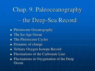
Chap. 9. Paleoceanography – the Deep-Sea Record

1. Chap. 9. Paleoceanography – the Deep-Sea Record • Pleistocene Oceanography • The Ice Age Ocean • The Pleistocene Cycles • Dynamic of change • Tertiary Oxygen Isotope Record • Fluctuations of the Carbonate Line • Fluctuations in Oxygenation of the Deep Ocean

2. 9.1 Background • Beginning in 1968, an enormous amount of effort in this subject, especially through the work of the CLIMAP group in Pleistocene oceanography, and through the extensive drilling in the deep sea by Glomar Challenger. • About 1 million years to the past 100 million years Fig.9.1 Recovering the Pleistocene record by piston coring. The corer is a wide-diameter model; note the white sediment in the core nose. Note also that the core barrel was bent during the operation (on the upper end), Other equipment on deck: deep-sea camera frame (with protective grid), hydrophone for seismic profiling (wrapped on spool), box corer (aft). [SIO Eurydice Expedition 1975]

3. 9.2 The Ice Age Ocean 9.2.1 Why an Ice Age • Several glaciations were discovered, with warm intervals separating them. • How many such advances and retreats of continental ice were there? • What is the time-scale of these cycles? • How do the cycles relate to astronomical factors, that is, the rotation of the Earth and its paths around the Sun? • These questions were difficult to even attempt to answer from the land record: each succeeding glaciation erased many of the traces of the previous one. • The study of long cores from the deep sea floor opened new possibilities.

4. Why is there an ice age at all? • We do not know for sure. • It is colder during an ice age than before and after, so that the Earth heat budget is involved. • The budget is largely controlled by albedo and by the greenhouse effect. • Albedo was increased and greenhouse gases were decreased.

5. 9.2.2 Conditions in a Cold Ocean How did the ice age ocean differ from the present one? • Surface currents were stronger. • The ocean surface was cooler than today. • Some ocean regions cooled more than others, and the regional degree of change depends closely on the movement of boundaries of climatic zones.

6. Surface currents were stronger. • Surface currents are driven by winds, and winds depend on horizontal temperature gradients. • With the ice rim and the polar front much closer to the Equator, the temperature difference between ice (0°C or less)and the tropics (≈25°C) was compressed into a much shorter distance than now. • Hence the temperature gradient was greater, winds were stronger, and so were ocean currents. • Equatorial upwelling was intensified as a consequence, and also coastal upwelling. • Thus, at the same time that fertility decreased in high latitudes, due to ice cover, it increased in mid-latitudes (because of intensified mixing) and in the subtropics (due to upwelling).

7. The ocean surface was cooler than today. • With a substantial part of northern continents and seas under ice, the Earth reflected the Sun's radiation more readily (had a higher albedo) than today, hence, it absorbed less of the radiation and its atmosphere was cooler. • A cold atmosphere holds less water than a warm one and large areas on land therefore were drier than today: Dry areas (such as grasslands and deserts) reflect more sunlight than wet ones (such as forests). • A more fertile ocean would be slightly more reflective than a clear dark blue one with less algal growth. • All these factors favored reflection of the Sun's radiation back into space, and hence favored cooling.

8. Table 9.1 albedo values of ocean and land surface

9. Some ocean regions cooled more than others, and the regional degree of change depends closely on the movement of boundaries of climatic zones. • If, for example, an area is near the boundary of subtropics and temperate belt, it will then belong alternately to one or the other zone. • Thus, here the changes are substantial. • Conversely, changes can be minimal in the center of tropical or subtropical climatic regions. • For example, Korea!

10. 9.2.3 The 18K Map Fig.9.2 Approximate distribution of sea surface temperatures for northern hemisphere summer, during the last ice age maximum (about 18000 years ago;"18K map"). Note the extent and thickness of ice. [CLIMAP Project Members, 1976, Science 191:1131, simplified]

11. From the information shown in 18K map, the ice age ocean 18,000 years ago was characterized by: • Increased thermal gradients along polar fronts, especially in the North Atlantic and Antarctic. • Equatorward displacement of polar frontal systems

12. General cooling of most surface waters, by about 2.3°C, on the average. • Increased upwelling along the Equator in Pacific and Atlantic. • Increased coastal upwelling and strenthening of eastern boundary currents • Nearly stable positions and temperatures of the central gyres in the major ocean basins.

13. 9.2.4 Pulsed Deglaciation • It took between 7000 and 8000 years, approximately, to reduce the ice masses to something like today. • The sea level rose some 120 m. • Recent detailed work on corals in Barbados confirmed earlier indications that deglaciation occurred in pulses or steps. Fig.9.3 Rate and timing of glacial meltwater discharge compared with subarctic summer insolation. Discharge calculated from a depth-versus-age curve for Barbados corals (A. palmata). Heavy line time scale based on radiocarbon dating; thin line time and colleagues, Nature 1990, 345: 405;dashed line summer insolation at 60°N, based on calculations by A. Berger.

14. Two major pulses • Step 1; 13.5~12.5 ka (Termination Ia) • Step 2; 11~9.5 kyrs (Termination Ib) • Agrees exactly with two major warming steps known from northern Europe

15. Comparison with the summer insolation curve at high northern latitudes suggests that unusually warm summers are responsible for initiating melting.

16. Younger Dryas • The retreat of the polar front in the North Atlantic also tool place in the discontinuous manner. • A substantial re-advance of this front occurred during the Younger Dryas, between 11,000 and 10,000 radiocarbon years. • According to ice core measurements, some 12,800 and 11,700 calendar years. • The origin is entirely unknown …. Meteorites?

17. 9.3 The Pleistocene Cycles 9.3.1 The Evidence • The Pleistocene record shows a long series of alternating climatic states. • The cycles express themselves as fluctuations in faunal and floral composition, in the abundance of carbonate, and in the content of δ18O of foraminiferal shells and in other properties. Fig9.4 a-c. The Pleistocene record in deep sea sediments. a Carbonate cycles of the eastern Pacific, magnetically dated b G. Menardii pulses (left) and transfer temperature cycle (right) compared with oxygen isotope stratigraphy, Caribbean Sea c Dissolution cycles compared with oxygen isotope stratigraphy, western Pacific

18. 9.3.2 The Carbonate Cycles of the equatorial Pacific • Dissolution cycles • high dissolution in interglacials (low CaCO3 values) • low dissolution in glacial (high CaCO3 values). • Productivity variations play a secondary role in producing the cycles.

19. Fluctuation of the sea level must be important. • During low sea level, shelves are exposed. • There is no place for carbonate to go except onto the deep sea floor. • Conversely, during interglacials the high sea level allows shallow water carbonates to build up. • This carbonate is extracted from the ocean, and is no longer available for deposition on the deep sea floor.

20. The Atlantic carbonate cycles are largely dilution cycles. • During glacials the supply of terrigenous materials from the continents surrounding the Atlantic is greatly increased. • In high latitudes the activity of the ice grinds up enormous masses of rock. • The plant cover, which protects soil from erosion, is less dense. • In the subtropics deserts are wide-spread, delivering dust. • Flash floods in semi-arid regions are efficient conveyors of huge amounts of material. • The tropical rain forest is much reduced, and semi-arid regions are expanded. • The shelves are exposed, and subject to erosion. • All these factors contribute to the glacial increase of terrigenous deposition rates. • As the supply of terrigenous material increases, of course, the proportion of carbonate in pelagic sediments decreased accordingly.

21. 9.3.3 The Faunal (and Floral) Cycles • Warm-cold cycles; abundance of warm-water and cold-water planktonic foraminifera. • They are well defined in their amplitudes. • They tend to avoid intermediate values, suggesting that there are two prefered states: warm, and cold, but not in between. • The present time rather unusual in being so warm: for the last one half million years or so the climate was mostly much more severe.

22. 9.3.4 Oxygen Isotope Cycles • C. Emiliani (1955) from several long core taken in the Caribbean and North Atlantic • Species with the lowest δ18O, reasoning that these species must live in shallow water and therefore reflect surface water temperature. • The composition of seawater controls 18O/16O ratios. • During build-up of the ice, 18O stays preferentially in the ocean, increasing the 18O/16O ratio.

23. Loess Record in China: Drought-Wet Cycles • Glacial intervals are characterized by eolian dust deposits and interglacials by soil development. • Maximum wind supply occurred both during onset of glacials and during their maximum. • Such supply of dust by wind has implications for deep-sea sedimentation - perhaps (as dust brings phosphate and iron) even for productivity in the ocean.

24. Loess in China

25. Loess Record in China: Drought-Wet Cycles Fig.9.5 a-d. Correlation of loess profiles from Xifeng (China, see inset) with marine δ18O record during the last 500000 years. a Loess profile, L loess; S soil b Same profile with refined ages of loess sedimentation based on correlation to eolian flux record in (C); c Eolian flux record of the North Pacific, Core V 21-146 (mg/cm2/kyr) from 3968 m water depth and with a distance of more than 300 km from the loess source area; δ18O-Stratigraphy (‰, PDB) of this core, used for dating.[S. a. Hovan et al. 1989, Nature, 340:296]

26. 9.3.5 Milankovitch Cycles and Dating • The isotopic variations clearly indicate some sort of regular cycling such as could be produced by the Milankovitch mechanism which invokes regular variations in the Earth's orbital parameters as a cause for the succession of ice ages separated by warm periods. • The hypothesis of Milutin Milankovitch (1879-1958) states that long-term fluctuations in the radiocarbon received from the Sun, during summer seasons, in the high latitudes of the northern hemisphere, have controlled the occurrence of ice ages over the last 600,000 years.

27. A time-scale for the isotopic variations was needed. • C-14 dating of the uppermost portion of the record, and extrapolation downward is not very reliable. • Uranium dating of corals • Magnetic reversals

28. Precession • The axis is not stationary in space, and does not always point to the North Star as at the present. • Instead, it describes a circle, of which the North Star is one point. • The circle is completed once in about 21,000 years.

29. Obliquity • The inclination of the Earth's axis to the plane of its orbit changed through time. • It is 66 1/2° at present, but varies between about 65° and 68° once in 41000 years. • High obliquity obviously means warm summers and cold winters.

30. Eccentricity • The earth's orbit about the sun is not a circle but an ellipse. • The ratio between the long and the short axis varies through time. • One cycle takes about 100000 years.

31. Fig.9.6 The Croll-Milankovith Theory of the ice ages, and its test. upper 3 panels. Curves showing orbital parameters as calculated by A. L. Berger[ in M. A. Kominz et al., 1979, Earth Planet Sci. Lett. 45:392]. 1m=100000yrs. The eccentricity is the deviation of the orbit from a perfect circle, for which e-0. The eccentricity varies with a period near 100000 years. The precession parameter is a function of both the position of perihelion (point of Earth's orbit which is closest to the Sun) with respect to the equinoxes (day = night positions) and the eccentricity of the orbit (which makes the difference of equinox and perihelion significant in terms of seasonal irradiation). The periodicity of the precession parameter is near 21000years. Note the small variations during times of low eccentricity. The obliquity is the  angle of the Earth's axis, with respect to the vertical on the orbital plane (inset, lower right). It varies with a period of 41000 years. Lower panel curves showing the orbital periodicities contained in the oxygen isotope record in a subantarctic deep sea core. The solid line in the middle represents the original isotope record; superimposed (dotted line) is the eccentricity variation. Top curve 23000- year component extracted from the isotope record by band pass filter (a statistical method); bottom curve obliquity component extracted in a similar fashion. Inset right illustrates obliquity.[J. D. Hays et al., 1976, Science 194: 1121] M. Milankovithch's classical paper was published in 1920; Theorie mathematique des phenomenes thermiques produits par la radiation solaire, Gauthier-Villars, Paris, 339 pp.

32. 9.3.6 A Change in Tune • The stabilization of the maximum amplitude and the "saw-tooth" shape of the curve. • Neither of these properties is at all understood, because the dynamics of atmosphere-ocean interaction cannot yet be modeled on the time scale which is appropriate here. Fig.9.7 Oxygen isotope record of G. sacculifer, ODP Site 806, western equatorial Pacific. Age scale based on counting obliquity cycles extracted from the record (and set at 42000 years; see Fig.9.6). 5, 9,15, etc Isotope stages; o15, o30, 045 position of crests of obliquity-related cycles; MPR, eccentricity-dominated-B/M, Brunhes-Matuyama boundry. at 790kyrs. A. B. C. major cyclostratigraphic subdivisions, each with 15 obliquity cycles, where o15 = 625000 yrs; "Milankovitch Epoch" o15-o30 "Croll Epoch"; o30-o45 "Laplace Epoch".

33. It is interesting how much the 100,000-year eccentricity cycle dominates the scene throughout the last 900,000 years. • The lower half of the Quarternary essentially has no 100,000 years cycles at all. • The δ18O fluctuations are entirely dominated by the obliquity cycle.

34. 9.4 The Carbon Connection 9.4.1 A Major Discovery • The reconstruction of the composition of the Pleistocene atmosphere from ice cores • Glacial CO2 concentrations in air were lower than interglacial ones by a factor of 1.5. Fig.9.8 Carbon dioxide concentrations in the Vostok ice core from Antarctica(J. M. Bamola et al., 1987, Nature 329:408), compared with a productivity-related δ13C signal from the eastern tropical Pacific (N. J. Shackleton et al.,  1983 Nature 306:319). The signal plotted is the difference in δ13C of a planktonic and a benthic species, which constitutes a proxy for the nutrient content in deep water. The time scale of the CO2 record was adjusted using the deuterium record in the ice and the δ13C record in the sediments.

35. Methane gas also was measured; the fluctuations are similar to those of carbon dioxide. • The observed amplitude of CO2 variation correspond to a greenhouse effect of between 1 and 2 ˚C.

36. 9.4.2 Paleoproductivity • phosphate is added to the ocean (increased nutrient supply) • CO2-depleted surface waters • reduced atmospheric CO2 • Increase in δ13C of DIC • linking pCO2 and the difference in δ13C of planktonic and benthic foraminifers Fig.9.9 Sketch of a mechanism linking productivity to the carbon dioxide content of the atmosphere. According to W. S. Broecker (ocean chemistry during glacial time. Geochim Cosmochim Acta, 46, 1689-1705, 1982) when phosphate is added to the ocean a new equilibrium is established, with surface waters being more CO2-depleted than before. This then reduces atmospheric CO2. An increased in nutrient supply, through bio-pumping, also increases δ13C of the dissolved inorganic the carbon in surface water (by preferential removal of 12C into organic matter which sinks). Thus, the biopump mechanism provides a simple conceptual model linking pCO2 and the difference in δ13C of planktonic and benthic foraminifers (as shown in Fig.9.8)

37. Biological Pumping • The corresponding difference in δ13C, which is picked up in shells of planktonic and benthic foraminifers, is a measure of the intensity of the fractionation resulting from the biological pumping. • This intensity depends entirely on the nutrient content of deep ocean waters.

38. The bio-pump model for changing CO2 content of the atmosphere implies higher productivity of the ocean during glacial time. • Good independent evidence that productivity was higher during glacials. • Off NW Africa, the rate of burial of organic carbon was higher during glacials. • The cause is increased eastern boundary upwelling due to an increase in trade winds and monsoonal winds.

39. Fig.9.10 a, b. Paleoproductivity reconstructions for the late Pleistocene, off NW Africa. a Oxygen isotopes, sedimentation rates, and organic matter content in Meteor core 12392. Right resulting paleoproductivity estimates. Isotope stages as in Figs.9.7. and 9.4 c. (1 Holocene; 2-4 last glaciation; 5a-e last inetglacial; 6 earlier glaciation). b Importance of wind in producing changes in upwelling, as seen in correlation with dust supply (from which the strength of the wind is calculated

40. The general increase in productivity may have resulted in the burial of sufficient additional carbon to pull down the CO2 content significantly. • During times of low sea level, carbonate deposition would have been greatly decreased on the shelves. • This would have increased the carbonate ion content of the ocean and hence the "alkalinity" of the ocean. • This allows the ocean to retain a large share of the total CO2 in the system.

41. 9.4.3 The Long-Range View • Not just the ocean's exchange with the atmosphere, but also the weathering of silicates on land, and the input of CO2 from volcanism • The weathering process can be summarily described by the formula • CO2 + CaSiO3 → CaCO3 + SiO2 • which shows long-term uptake of CO2 from the atmosphere. • Long-term decrease in CO2 through mountain building and deep erosion. • Mountain-building and sea level drop proceeded all through the late Tertiary. • Changing ratio of strontium isotopes within marine sediments • One possible cause for the onset of the ice ages: a drop in atmospheric CO2 as a long-term trend within the late Tertiary

42. 9.5 Tertiary Oxygen Isotope Record 9.5.1 Trends and Events: Oxygen Isotopes • An overall cooling trend since the Cretaceous, from the increase of oxygen-18 in benthic foraminifera.

43. Tertiary Oceans : the Cooling Planet Fig.9.11 a, b. Schematic diagram of the planetary cooling trend in the Cenozoic. a Generalized sea level curve, showing overall regression (J. Thiede et al., 1992, Polarforschung 61[1]; 1; based on a compilation by L. A. Frakes). b oxygen isotopic composition of planktonic and benthic foraminifera in deep-sea sediments. Vertical lines marked MM and EO show approximate position of major cooling steps, which involve high latitudes and deep ocean water masses

44. The oxygen isotopic composition of planktonic and of benthic foraminifera shows separate trends for low latitudes, but similar trends for high latitudes. • Thus, the Tertiary cooling trend is indeed largely a high latitude (and deep water) phenomenon. • In general, then, temperature gradients must have increased throughout the Tertiary, especially since the end of the Oligocene some 20 to 25 million years ago. • Wind speed depends strongly on temperature gradients. • If so, winds and their offspring, the surface currents, greatly increased since the Oligocene, as did coastal and mid-ocean upwelling. • Direct evidence is found in the increasing diatom supply, both in the northern North Pacific and around the Antarctic, during the Late Tertiary.

45. 9.5.2 The Great Partitioning • All through the Tertiary, changes in geography due to plate motions affect the configuration of exchange between ocean basins. • The gateways control access to the Arctic Ocean (east and west of Greenland), connnect the global ocean along the Equator ("Tethys Ocean" between Africa and Eurasia, Panama Straits, Indonesian Seaway between Borneo and New Guinea), and control the evolution of the Circumpolar Current (Tasmanian Passage, Drake Passage).

46. The Great Partitioning Fig.9.12 Geography of the middle Eocene (ca 45 Ma) and major critical valve points for ocean circulation. Tropical valves are closing (filled rectangles), high latitude valves and opening up (open rectangles) throughout the Cenozoic.[Base map from B. U. Haq, Oceanologica Acta, 4 Suppl.:71]

47. The Great Partitioning • The difference from the present ocean to the Eocene ocean 45 million years ago consists mainly in the tropical gateways and the opening of the poleward ones. • One of the most fascinating is the drying out of the Mediterranean between about 6 to 5 million years ago. • Huge amount of salt were deposited at that time, so much that the salinity of the global ocean may have been reduced by 6 %. • Messinian Crisis

48. 9.5.3 The Grand Asymmetries • What are the consequences for ocean circulation of the large-scale valve switch executed by continents moving away from Antarctica? • Restricted Southern Ocean; cold box • The average ocean has to be cold. • Deep-sea and cold-water faunas become global, while tropical ones become more provincial. • Tertiary ocean history; the increased displacement of the intertropical convergence zone (ITCZ, the heat equator) to the north of Equator.

49. Several causes • The whitening of the Antarctic continent; the effect of pushing climatic zones northward • The northward movement of large continental masses which sets up monsoonal regimes favorable for northward heat transfer • The uplift of Tibet and the Himalayas; strengthening of monsoons and an increase in weathering • The peculiar geographic configuration in both major oceans, Atlantic and Pacific, which provides for deflection of westward-flowing equatorial currents, sending them northward to strenghen the Gulf Stream and the Kuroshio.

50. The Grand Asymmetries • The end result is that the southern hemisphere is robbed of heat by the northern hemisphere. • Glaciers in southern New Zealand are in walking distance from the seashore, at a latitude which corresponds to that of the vineyards of Bordeaux!