Download

1 / 17
220 likes | 1.01k Vues
Determination of the rate law. Isolation method: v = k [A] a [B] b -----> v = k ’[B] b Method of initial rates (often used in conjunction with the isolation method): v = k [A] a at the beginning of the reaction v 0 = k [A 0 ] a

E N D
Determination of the rate law • Isolation method: v = k [A]a[B]b -----> v = k’[B]b • Method of initial rates (often used in conjunction with the isolation method): v= k [A]a at the beginning of the reaction v0 = k [A0]a taking logarithms gives: logv0 = log k + a log[A0] therefore the plot of the logarithms of the initial rates against the logarithms of the initial concentrations of A should be a straight line with the slope a (the order of the reaction).
Self-test 22.3: The initial rate of a reaction depended on the concentration of a substance B as follows: [B]0/(mmol L-1) 5.0 8.2 17 30 v0/(10-7 mol L-1s-1) 3.6 9.6 41 130 Determine the order of the reaction with respect to B and calculate the rate constant. Solution: Log([B]0) -2.30 -2.086 -1.770 -1.523 Log(v0) -6.444 -6.018 -5.387 -4.886
22.3 Integrated rate law • First order reaction: A Product The solution of the above differential equation is: or: [A] = [A]0e-kt • In a first order reaction, the concentration of reactants decreases exponentially in time.
Self-test 22.4:In a particular experiment, it was found that the concentration of N2O5 in liquid bromine varied with time as follows: t/s 0 200 400 600 1000 [N2O5]/(mol L-1) 0.110 0.073 0.048 0.032 0.014 confirm that the reaction is first-order in N2O5 and determine the rate constant. Solution:To confirm whether a reaction is first order, plot ln([A]/[A]0) against time. First order reaction should yield a straight line! t/s 0 200 400 600 1000 ln([A]/[A]0) 0 -0.410 -0.829 -1.23 -2.06
Half-lives and time constant • For the first order reaction, the half-live equals: therefore, is independent of the initial concentration. • Time constant, , the time required for the concentration of a reactant to fall to 1/e of its initial value. for the first order reaction.
Second order reactions • Case 1: second-order rate law: (e.g. A → P) • Can one use A + A → P to represent the above process? • The integrated solution for the above function is: or • The plot of 1/[A] against t is a straight line with the slope k.
Case 2: The rate law (e.g. A + B → Product) • The integrated solution (to be derived on chalk board) is :
22.4 Reactions approaching equilibrium Case 1:First order reactions: A → B v = k [A] B → A v = k’ [B] the net rate change for A is therefore if [B]0 = 0, one has [A] + [B] = [A]0 at all time. the integrated solution for the above equation is [A] = As t → ∞, the concentrations reach their equilibrium values: [A]eq = [B]eq = [A]0 – [A]eq =
The equilibrium constant can be calculated as K = thus: • In a simple way, at the equilibrium point there will be no net change and thus the forward reaction rate is equal to the reverse: k[A]eq = k’ [B]eq thus the above equation bridges the thermodynamic quantities and reaction rates through equilibrium constant. • For a general reaction scheme with multiple reversible steps:
Determining rate constants with relaxation method • After applying a perturbation, the system (A ↔ B) may have a new equilibrium state. Assuming the distance between the current state and the new equilibrium state is x, one gets [A] = [A]eq + x; [B] = [B]eq - x; Because one gets dx/dt = - (ka + kb)x therefore is called the relaxation time
Example 22.4: The H2O(l) ↔ H+(aq) + OH-(aq) equilibrium relaxes in 37 μs at 298 K and pKw = 14.0. Calculate the rate constants for the forward and backward reactions. Solution: the net rate of ionization of H2O is we write [H2O] = [H2O]eq + x; [H+] = [H+]eq – x; [OH-] = [OH-]eq – x and obtain: Because x is small, k2x2 can be ignored, so Because k1[H2O]eq = k2[H+]eq[OH-]eq at equilibrium condition = = hence k2= 1.4 x 10¹¹ L mol-1 s-1 k1 = 2.4 x 10⁻⁵ s-1
Self-test 22.5: Derive an expression for the relaxation time of a concentration when the reaction A + B ↔ C + D is second-order in both directions.
22.5 The temperature dependence of reaction rates • Arrhenius equation: A is the pre-exponential factor; Ea is the activation energy. The two quantities, A and Ea, are called Arrhenius parameters. • In an alternative expression lnk = lnA - one can see that the plot of lnk against 1/T gives a straight line.
25 20 15 Series1 10 5 0 0 0.0005 0.001 0.0015 0.002 0.0025 0.003 0.0035 Example: Determining the Arrhenius parameters from the following data: T/K 300 350 400 450 500 k(L mol-1s-1) 7.9x10⁶ 3.0x10⁷ 7.9x10⁷ 1.7x10⁸ 3.2x10⁸ Solution: 1/T (K-1) 0.00333 0.00286 0.0025 0.00222 0.002 lnk (L mol-1s-1) 15.88 17.22 18.19 18.95 19.58 The slope of the above plotted straight line is –Ea/R, so Ea = 23 kJ mol-1. The intersection of the straight line with y-axis is lnA, so A = 8x10¹⁰ L mol-1s-1
The interpretation of the Arrhenius parameters • Reaction coordinate: the collection of motions such as changes in interatomic distance, bond angles, etc. • Activated complex • Transition state • For bimolecular reactions, the activation energy is the minimum kinetic energy that reactants must have in order to form products.
Applications of the Arrhenius principle Temperature jump-relaxation method: consider a simple first order reaction: A ↔ B at equilibrium: After the temperature jump the system has a new equilibrium state. Assuming the distance between the current state and the new equilibrium state is x, one gets [A] = [A]eq + x; [B] = [B]eq - x;