Objective Analysis and Data Assimilation
Objective Analysis and Data Assimilation. Exploring the Components of an NWP System. Objective Analysis/Data Assimilation. Numerical weather models are generally solved on a three-dimensional grid Observations are scattered in three dimensions

Objective Analysis and Data Assimilation
E N D
Presentation Transcript
Objective Analysis/Data Assimilation Numerical weather models are generally solved on a three-dimensional grid Observations are scattered in three dimensions Need to interpolate observations to grid points and to insure that the various fields are consistent and physically plausible (e.g., most of the atmosphere in hydrostatic and gradient wind balance).
Objective Analysis/Data Assimilation Often starts with a “first guess”, usually the gridded forecast from an earlier run (frequently a run starting 6 hr earlier) This first guess is then modified by the observations. Adjustments are made to insure proper balance. Objective Analysis/Data Assimilation produces what is known as the model initialization, the starting point of the numerical simulation.
Objective Analysis Definition The graphic to the right depicts the basic problem of objective analysis, namely that we have irregularly spaced observations that must provide values for points on a regularly spaced grid. (Red dots represent observations and blue dots are grid points.) Objective analysis in NWP is the process of interpolating observed values onto the grid points used by the model in order to define the initial conditions of the atmosphere. Why isn’t this just a simple exercise in mathematical interpolation? There are several answers to this question.
Objective Analysis Definition 1.We can use our knowledge of atmospheric behavior to infer additional information from the data available in the area. For example, we can use balance relationships such as geostrophy or mass continuity to introduce dynamical consistency into the analysis. If we use one type of data to improve the analysis of another, then the analysis is said to be multivariate (e.g., height data can be used to help the analysis of winds).
Objective Analysis Definition 2. We can adjust the analysis procedure to filter out scales of motion that can’t be forecast by the model being used. For example, small mesoscale circulations represented in the observations may need to be smoothed out in an analysis for a global model.
Objective Analysis Definition 3. We can make use of a first guess field or background field provided by an earlier forecast from the same model. The blending of the background fields and the observations in the objective analysis process is especially important in data sparse areas. It allows us to avoid extrapolation of observation values into regions distant from the observation sites. The background field can also provide detail (such as frontal locations that exist between observations). Using a background field also helps to introduce dynamical consistency between the analysis and the model. In other words, that part of the analysis that comes from the background field is already consistent with the physical (dynamic) relationships implied by the equations used in the model.
Objective Analysis Definition 4. We can also make use of our knowledge of the probable errors associated with each observation. We can weight the reliability of each type of observation based on past records of accuracy.
In this section, we will examine a fundamental objective analysis equation in worded form in order to illustrate the basic principles that contribute to a numerical meteorological analysis. In simplest terms, the objective analysis equation attempts to determine the value of a particular meteorological variable at a particular grid point (at a particular valid time). In words, the analysis equation can be expressed as shown below. Analysis Equation
The Importance of the Background Field In the simplest kind of objective analysis scheme, the background values would not be used and the analysis would be based solely on new observations. In this case the equation would become: The observations themselves would be interpolated to the grid point by calculating a weighted average of the data. (One type of weight, for example, is proportional to the distance of the data from the grid point. The farther an observation is from the grid point, the less weight it gets.) If a grid point has no nearby observations, the simple scheme described here is in trouble!
Suppose we had a surface low along a coastline and the only observations (in red) were over the land. In order to obtain an analysis value at grid point “A”, a simple objective analysis scheme would have to extrapolate from the available data. Since there are no nearby data to the west of point “A”, an extrapolated value would reflect the decrease in pressure towards the coastline in the available data. Therefore the analyzed pressure at point “A” would be in the neighborhood of 974 hPa (whereas the correct value would be closer to 986 hPa)! So how can we solve this problem of data void areas? Analysis Equation
Analysis Equation One solution is to start our analysis using a short-range forecast of the same field from an earlier run of some NWP model (usually the same one that will use the analysis). If the forecast period is fairly short, say 3-6 hours, then very little error will have accumulated. This forecast (the background field, or first guess) will provide a much better estimate of the atmosphere over data sparse regions than would an extrapolation of distant observations. In the previous example, a 6-hr forecast of the surface low might produce an estimate at point “A” that would be in error by 2-4 hPa rather than 12 hPa.
Analysis Equation The first place the background field is used is in calculating the “correction”values for each observation site. This correction value, known as the observation increment, is the difference between the observed value and an interpolated background value for that observation point. In other words, the “new information” that will be analyzed to the grid point are the changes that the observations make to the background field, rather than the observations themselves.
Analysis Equation The background field is also used in the final step of the analysis in that the final analysis value is defined as the background value plus the weighted sum of observation increments (corrections). The use of the background field ensures that the analysis will blend smoothly from regions with good data to regions with no or sparse data (where the background field is allowed to dominate in determining the analysis value). Because this provides a better analysis of data sparse regions than an extrapolation of the observations, all objective analysis schemes used by NWP use background fields.
Analysis Equation For this reason, a very high priority in improving objective analysis is to improve the background field. Two ways to do this include: • We can set up a data assimilation procedure that allows us to make a sequence of short-range forecasts to provide background fields rather than one longer-range forecast. • We can improve the forecast model! There is a very interdependent relationship between an analysis and the model that uses it: The better the analysis, the better the forecast. The better the forecast model, the better the background field , therefore, the better the analysis.
Analysis Equation - Weight Factor Each observation increment is weighted based on its perceived accuracy and validity. The biggest difference among objective analysis schemes is how the weighting of observation increments is done.
Interpolating a Surface From Sampled Point Data
Interpolating a Surface From Sampled Point Data • Assumes a continuous surface that is sampled • Interpolation • Estimating the attribute values of locations that are within the range of available data using known data values • Extrapolation • Estimating the attribute values of locations outside the range of available data using known data values
Estimating a point here:interpolation Sample data Interpolating a Surface From Sampled Point Data Interpolation
Sample data Estimating a point here:extrapolation Interpolating a Surface From Sampled Point Data Extrapolation
Interpolating a Surface From Sampled Point Data • Sampling Strategies for Interpolation Regular Sampling Random Sampling
If A = 8 feet and B = 4 feet then C = (8 + 4) / 2 = 6 feet Sample elevation data A C B Elevation profile Interpolating a Surface From Sampled Point Data Linear Interpolation
Sample elevation data Often results in a more realistic interpolation but estimating missing data values is more complex A C B Elevation profile Interpolating a Surface From Sampled Point Data Non-Linear Interpolation
Sample data Interpolating a Surface From Sampled Point Data Global Interpolation Uses all known sample points to estimate a value at an unsampled location
Sample data Uses a local neighborhood to estimate value, i.e. closest n number of points, or within a given search radius Interpolating a Surface From Sampled Point Data Local Interpolation Uses a neighborhood of sample points to estimate a value at an unsampled location
Trend Surface • Global method • Inexact • Can be linear or non-linear • predicting a z elevation value [dependent variable] with x and y location values [independent variables]
z z = b0 + b1x + e x Trend Surface 1st Order Trend Surface In one dimension:z varies as a linear function ofx
z y z = b0 + b1x + b2y + e x Trend Surface 1st Order Trend Surface In two dimensions:z varies as a linear function of xandy
Inverse Distance Weighted • Local method • Exact • Can be linear or non-linear The weight (influence) of a sampled data value is inversely proportional to its distance from the estimated value
100 IDW: Closest 3 neighbors, r = 2 4 3 160 2 200 Inverse Distance Weighted(Example)
Weights A BC 1 / (42) = .0625 1 / (32) = .1111 1 / (22) = .2500 A = 100 4 B = 160 3 2 C = 200 Inverse Distance Weighted(Example)
Weights Weights * Value A BC 1 / (42) = .0625 1 / (32) = .1111 1 / (22) = .2500 .0625 * 100 = 6.25 .1111 * 160 = 17.76 .2500 * 200 = 50.00 Total = .4236 A = 100 4 6.25 +17.76 + 50.00 = 74.01 B = 160 3 74.01 / .4236 = 175 2 C = 200 Inverse Distance Weighted(Example)

