Chapter 4 Exploiting Instruction-Level Parallelism with Software Approaches

1. Chapter 4Exploiting Instruction-Level Parallelism with Software Approaches

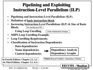
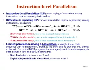
2. Basic Compiler Techniques for Exposing • Basic pipeline scheduling and loop unrolling • To keep a pipeline full, parallelism among instructions must be exploited by finding sequences of unrelated instructions that can be overlapped in the pipeline. • A compiler’s ability to perform such kind of scheduling depends on both the amount of ILP available in the program and on the latencies of the functional units in the pipeline. • To avoid a pipeline stall, a dependent instruction must be separated from the source instruction by a distance in clock cycles equal to the pipeline latency of that source instruction..

3. Scheduling and Loop Unrolling • Basic assumptions: • The latencies of the FP unit Inst. producing result Inst. Using result Latency FP ALU op Another FP ALU op 3 FP ALU op Store double 2 Load double FP ALU op 1 Load double Store double 0 • The branch delay of the pipeline implementation is 1 delay slot. • The functional units are fully pipelined or replicated such that no structural hazards can occur

4. Loop Unrolling by Compilers • Example: for (j=1, j<= 1000, j++) x[j]=x[j]+s; • Assume R1 initially holds the highest address of the first element and 8(R2) holds the last element. Loop: L.D F0, 0(R1) ADD.D F4, F0, F2 S.D F4, 0(R1) DADDUI R1, R1, #-8 BNE R1, R2,Loop • Performance of scheduled code with loop unrolling.

5. Performance of Unscheduled Code without Loop Unrolling Clock cycle issued Loop: L.D F0, 0(R1) 1 stall 2 ADD.D F4, F0, F2 3 stall 4 stall 5 S.D F4, 0(R1) 6 DADDUI R1, R1, #-8 7 stall 8 BNE R1, R2,Loop 9 stall 10 • Need 10 cycles per result

6. Performance of Scheduled Code without Loop Unrolling Loop: L.D F0, 0(R1) DADDUI R1, R1, #-8 ADD.D F4, F0, F2 stall BNE R1, R2,Loop ; delay branch S.D F4, 8(R1) • Need 6 cycles per result

7. Performance of Unscheduled Code with Loop Unrolling • Unroll the loop 4 iterations Loop: L.D F0, 0(R1) ADD.D F4, F0, F2 S.D F4, 0(R1) L.D F6, -8(R1) ADD.D F8, F6, F2 S.D F8, -8(R1) L.D F10, -16(R1) ADD.D F12, F10, F2 S.D F12, -16(R1) L.D F14, -24(R1) ADD.D F16, F14, F2 S.D F16, -24(R1) DADDUI R1, R1, #--32 BNE R1, R1, Loop • Needs 7 cycles per result

8. Performance of Scheduled Code with Loop Unrolling Loop: L.D F0, 0(R1) L.D F6, -8(R1) L.D F10, -16(R1) L.D F14, -24(R1) ADD.D F4, F0, F2 ADD.D F8, F6, F2 ADD.D F12, F10, F2 ADD.D F16, F14, F2 S.D F4, 0(R1) S.D F8, -8(R1) DADDUI R1, R1, #--32 S.D F12, 16(R1) BNE R1, R1, Loop S.D F16, 8(R1) • Need 3.5 cycles per result

9. Using Loop Unrolling and Pipeline Scheduling with Static Multiple Issue • Fig. 4.2 on page 313

10. Static Branch Prediction • For a compiler to effectively schedule the code such as for scheduling branch delay slot, we need to statically predict the behavior of branches. • Static branch prediction used in a compiler LD R1, 0(R2) DSUBU R1, R1, R3 BEQZ R1, L OR R4, R5, R6 DADDU R10, R4, R3 L: DADDU R7, R8, R9 • If the BEQZ was almost always taken and the value of R7 was not needed on the fall through path, DADDU can be moved to the position after LD. • If it is rarely taken and the value of R4 was not needed on the taken path, OR can be moved to the position after LD.

11. Branch Behavior in Programs • Program behavior • Average frequency of taken branches : 67% • 60% of the forward branches are taken. • 85% of the backward branches are taken • Methods for statically branch prediction • By examination of the program behavior • Predict-taken (mis-prediction rate: 9%~59%). • Predict-forward-untaken and backward taken. • The above two approaches combined mis-prediction rate is 30%~40%. • By the use of profile information collected from earlier runs of the program.

12. Mis-prediction Rate for a Profile-Based Predictor

13. Comparison between Profile-Based and Predict-Taken

14. The Basic VLIW Approach • VLIW uses multiple, independent functional units. • Multiple, independent instructions are issued by processing a large instruction package that consists of multiple operations. • A VLIW instruction might include one integer/branch instruction, two memory references, and two floating-point operations. • If each operation requires a 16 to 24 bits field, the length of each VLIW instruction is of 112 to 168 bits. • Performance of VLIW

15. Scheduling of VLIW Instructions • Fig. 4.5 on page 318

16. Limitations to VLIW Implementation • Limitations • Technical problem • To generate enough straight-line code fragment requires ambitiously unrolling loops, which increases code size. • Poor code density • Whenever the instructions are not full, the unused functional units translate into wasted bits in the instruction encoding (only 60% full). • Logistical problem • Binary code compatibility; it depends on • Instruction set definition, • The detailed pipeline structure, including both functional units and their latencies. • Advantages of a superscalar processor over a VLIW processor • Little impact on code density. • Even unscheduled programs, or those compiled for older implementations, can be run.

17. Advanced Compiler Support for Exposing and Exploiting ILP • Exploiting Loop-Level Parallelism • Converting the loop-level parallelism into ILP • Software pipelining (Symbolic loop unrolling) • Global code scheduling

18. Loop-Level Parallelism • Concepts and techniques • Loop-level parallelism is normally analyzed at the source level while most ILP analysis is done once the instructions have been generated by the compiler. • The analysis of loop-level parallelism focuses on determining whether data accesses in later iterations are data dependent on data values produced in earlier iterations. • Example: for (i=1; i<=1000; i++) x[i]=x[i]+s; • Loop-carried data dependence: Dependence exists between different iterations of the loop. • A loop is parallel unless there is a cycle in the dependences. Therefore, a non-cycled loop-carried data dependence can be eliminated by code transformation.

19. Loop-Carried Data Dependence (1) • Example for (I=1; I<=100; I=I+1){ A[I+1] = A[I]+C[I]; /* S1 */ B[I+1] = B[I]+A[I+1]; /* s2 */ } • Dependence graph

20. Loop-Carried Data Dependence (2) • Example for (I=1; I<=100; I=I+1){ A[I] = A[I]+B[I]; /* S1 */ B[I+1] = C[I]+D[I]; /* s2 */ } • Code transformation A[1] = A[1] +B[1]; for (I=1; I<99; I=I+1){ B[I+1] = C[I]+D[I]; /* s2 */ A[I+1] = A[I+1]+B[I+1]; /* S1 */ } • Convert loop-carried data dependence into data dependence.

21. Loop-Carried Data Dependence (3) • True loop-carried data dependence are usually in the form of a recurrence. For (I=2; I<=100; I++){ Y[I] = Y[I-1] + Y[I]; } • Even true loop-carried data dependence has parallelism. For (I=6; I<=100; I++){ Y[I] = Y[I-5] + Y[I]; } • The first, second, …, five iterations are parallel.

22. Detecting and Eliminating Dependencies • Finding the dependences in a program is an important part of three tasks: • Good scheduling of code • Determining which loops might contain parallelism, and • Eliminating name dependence • Example • for (i=1; i<= 100; i++) { • A[i] = B[i] + C[i]; • D[i] = A[i] + E[i]; • } • Absence of loop-carried dependence, which implies existence of a large amount of parallelism.

23. Dependence Detection Problem • NP complete. • GCD test heuristic • Suppose we have stored to an array element with index value a*j+b and loaded from the same array with index value c*k+d, where j and k are the for-loop index variable that runs from m to n. A dependence exists if two conditions hold: • There are tow iteration indices, j and k, both within the limits of the for loop. • The loop stores into an array element indexed by a*j+b and later fetches from that same array element when it is indexed by c*k+d. That is, a*j+b=c*k+d. • Note, a,b,c, and d are generally unknown at compile time, making it impossible to tell if a dependence exists. • A simple and sufficient test for the absence of a dependence. If a loop-carried dependence exists, then GCD(c,a) must divide (d-b). That is if GCD(c,a) does not divide (d-b), no dependence is possible (Example on page 324).

24. Situations where Dependence Analysis Fails • When objects are referenced via pointers rather than array indices; • When array indexing is indirect through another array. • When a dependence may exist for some value of the inputs, but does not exist in actuality. • Others.

25. Eliminating Dependent Computations • Copy propagation DADDUI R1, R2, #4 DADDUI R1, R2, #4 to DADDUI R1, R2, #8 • Tree height reduction ADD R1, R2, R3 ADD R4, R1, R6 ADD R8, R4, R7 to ADD R1, R2, R3 ADD R4, R6, R7 ADD R8, R1, R4

26. Software Pipelining: Symbolic Loop Unrolling • Software pipelining is a technique for reorganizing loops such that each iteration in the software-pipelined code is made from instructions chosen from different iterations of the original loop. • A software-pipelined loop interleaves instructions from different loop iterations without unrolling the loop. • A software pipeline loop consists of a loop body, start-up code and clean-up code

27. Example Original loop Reorganized loop Loop: L.D F0, 0(R1) Loop: S.D F4, 16(R1) ADD.D F4, F0, F2 ADD.D F4, F0, F2 S.D F4, 0(R1) L.D F0, 0(R1) DADDUI R1, R1, #-8 DADDUI R1, R1, #-8 BNE R1, R2, Loop BNE R1, R2, Loop Iteration i: L.D F0, 0(R1) ADD.D F4, F0, F2 S.D F4, 0(R1) Iteration i+1: L.D F0, 0(R1) ADD.D F4, F0, F2 S.D F4, 0(R1) Iteration i+2: L.D F0, 0(R1) ADD.D F4, F0, F2 S.D F4, 0(R1)

28. Comparison between Software-Pipelining and Loop Unrolling • Software pipelining consumes less code space. • Loop unrolling reduces the overhead of the loop -- the branch and counter-updated code. • Software pipelining reduces the time when the loop is not running at peak speed to once per loop at the beginning and end.

29. Global Code Scheduling

30. Trace Scheduling: Focusing on Critical Path • Trace selection • Trace compaction • Bookkeeping code

31. Hardware Support for Exposing More Parallelism at Compile Time • The difficulty of uncovering more ILP at compile time ( due to unknown branch behavior) can be overcome by employing the following techniques: • Conditional or predicated instructions • Speculation • Static speculation performed by the compiler with hardware support. • Dynamic speculation performed by hardware using branch prediction to guide speculation process.

32. Conditional or Predicated instructions • Basic concept • An instruction refers to a condition, which is evaluated as part of the instruction execution. If the condition is true, the instruction is executed normally, otherwise, the execution continues as if it is a no-op. • The conditional instruction allows us to convert the control dependence present in the branch-based code sequence to a data dependence. • A conditional instruction can be used to speculatively move an instruction that is time critical • To use a conditional instruction successfully like the one in examples, we must ensure that the speculated instruction does not introduce an exception.

33. Conditional Move • Example on page 341

34. On Time Critical Path • Example on page 342 and 343

35. Example (Cont.)

36. Limiting Factors • The usefulness of conditional instructions is limited by several factors: • Conditional instructions that are annulled still take execution time. • Conditional instructions are most useful when the condition can be evaluated early. • The use of conditional instructions is limited when the control flow involves more than a simple alternative sequence. • Conditional instructions may have some speed penalty compared with unconditional instructions. • Machines that use conditional instruction • Alpha: Conditional move; • HP PA: Any register-register instruction; • SPARC: Conditional move; • ARM: All instructions.

37. Compiler Speculation with Hardware Support • In moving instructions across a branch the compiler must ensure that exception behavior is not changed and the dynamic data dependence remains the same. • The simplest case is that the compiler is conservative about what instructions it speculatively moves, and the exception behavior is unaffected. • Four methods • The hardware and OS cooperatively ignore exceptions for speculative instructions. • Speculative instructions that never raise exceptions are used, and checks are introduced to determine when an exception should occur. • Poison bits are attached to the result registers written by speculated instructions when the instruction cause exceptions. • The instruction results are buffered until it is certain that the instruction is no longer speculative.

38. Types of Exceptions • Two types of exceptions needs to be distinguished: • Exceptions cause program error, which indicates the program must be terminated. Ex., memory protection error. • Exceptions can be normally resumed, Ex., page faults. • Basic principles employed by the above mechanism: • Exceptions that can be resumed can be accepted and processed for speculative instructions just as if they are normal instruction. • Exceptions that indicate a program error should not occur in correct programs.

39. Hardware-Software Cooperation for Speculation • The hardware and OS simply • Handle all resumable exceptions when exception occurs, and • Return an undefined value for any exception that would cause termination. • If a normal instruction generate • terminating exception --> return an undefined value and program proceeds normally --> generate incorrect result, or • resumable exception --> accepted and handled accordingly --> program terminated normally. • If a speculative instruction generate • terminating exception --> return an undefined value --> a correct program will not use it --> the result is still correct. • resumable exception --> accepted and handled accordingly --> program terminated normally.

40. Example • On page 346 and 347

41. Speculative Instructions Never … (Method 2) • Example on page 347

42. Answer

43. Speculation with Poison Bits • A poison bit is added to every register and another bit is added to every instruction to indicate whether the instruction is speculative. • Three steps: • The poison bit is set whenever a speculative instruction results in a terminating exception; all other exceptions are handled immediately. • If a speculative instruction uses a register with a poison bit turned on, the destination register of the instruction simply has its poison bit turned on. • If a normal instruction attempts to use a register source with its poison bit turned on, the instruction causes a fault.

44. Example • On page 348

45. Hardware Support for Memory Reference Speculation • Moving load across stores is usually done when the compiler is certain the address do not conflict. • To support speculative load • A special check instruction to check for address conflict is placed at the original location of the load instruction. • When a speculated load is executed, the hardware saves the address of the accessed memory location. • If the value stored in the location is changed before check instruction, speculation fails. If not, it succeeds.

46. Hardware- versus Software-Based Speculation • Dynamic runtime disambiguation of memory addresses is conducive to speculate extensively. This allows us to move loads past stores at runtime. • Hardware-based speculation is better because hardware-based branch predictions is better than software-based branch prediction done at compile time. • Hardware-based speculation maintains a completely precise exception model. • Hardware-based speculation does not require bookkeeping codes. • Hardware-based speculation with dynamic scheduling does not require different code sequence for different implementation of an architecture to achieve good performance. • Compiler-based approaches can see further in the code sequence.

47. Concluding Remarks • Hardware and software approaches to increasing ILP tend to fuse together.