Instruction-Level Parallelism
Instruction-Level Parallelism. Outline. Instruction-Level Parallelism: Concepts and Challenges Overcoming Data Hazards with Dynamic Scheduling Reducing Branch cost with Dynamic Hardware Prediction High-Performance Instruction Delivery Hardware-Based Speculation

Instruction-Level Parallelism
E N D
Presentation Transcript
Outline • Instruction-Level Parallelism: Concepts and Challenges • Overcoming Data Hazards with Dynamic Scheduling • Reducing Branch cost with Dynamic Hardware Prediction • High-Performance Instruction Delivery • Hardware-Based Speculation • Studies of the Limitations of ILP
Introduction • Instruction-Level Parallelism (ILP): potential execution overlap among instructions • Instructions are executed in parallel • Pipeline supports a limited sense of ILP • This chapter introduces techniques to increase the amount of parallelism exploited among instructions • How to reduce the impact of data and control hazards • How to increase the ability of the processor to exploit parallelism
Approaches To Exploiting ILP • Hardware approach: focus of this chapter • Dynamic – running time • Dominate desktop and server markets • Pentium III and IV; • Software approach: focus of next chapter • Static – compiler time • Rely on compilers • Broader adoption in the embedded market • But include IA-64 and Intel’s Itanium
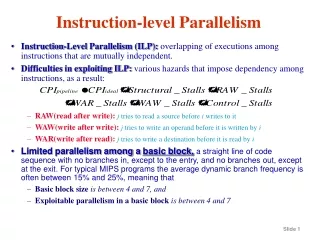
ILP within a Basic Block • Basic Block – Instructions between branch instructions • Instructions in a basic block are executed in sequence • Real code is a bunch of basic blocks connected by branch • Notice: dynamic branch frequency – between 15% and 25% • Basic block size between 6 and 7 instructions • May depend on each other (data dependence) • Therefore, probably little in the way of parallelism • To obtain substantial performance enhancement: ILP across multiple basic blocks • Easiest target is the loop • Exploit parallelism among iterations of a loop (loop-level parallelism)
Loop Level Parallelism (LLP) • Consider adding two 1000 element arrays • There is no dependence between data values produced in any iteration j and those needed in j+n for any j and n • Truly independent iterations • Independence means no stalls due to data hazards • Basic idea to convert LLP into ILP • Unroll the loop either statically by the compiler (next chapter) or dynamically by the hardware (this chapter) for (i=1; i<=1000, i=i+1) x[i] = x[i] + y[i]
Introduction • To exploit instruction-level parallelism we must determine which instructions can be executed in parallel. • If two instructions are independent, then • They can execute (parallel) simultaneously in a pipeline without stall • Assume no structural hazards • Their execution orders can be swapped • Dependent instructions must be executed in order, or partially overlapped in pipeline • Why to check dependence? • Determine how much parallelism exists, and how that parallelism can be exploited
Types of dependences Types of dependences • Data • Name • Control dependence
Data Dependence Analysis • i is data dependent on j if i uses a result produced by j • OR i uses a result produced by k and k depends on j (chain) • Dependence indicates a potential RAW hazard • Induce a hazard and stall? - depends on the pipeline organization • The possibility limits the performance • Order in which instructions must be executed • Sets a bound on how much parallelism can be exploited • Overcome data dependence • Maintain dependence but avoid a hazard – scheduling the code (HW,SW) • Eliminate a dependence by transforming the code (by compiler)
Data Dependence Example Loop: L.D F0, 0(R1) ADD.D F4, F0, F2 S.D F4, 0(R1) DADDUI R1, R1, #-8 BNE R1, R2, Loop If two instructions are data dependent, they cannot execute simultaneously or be completely overlapped.
Data Dependence through Memory Location • Dependences that flow through memory locations are more difficult to detect • Two Addresses may refer to the same location but look different • Example : 100(R4) and 20(R6) may be identical • The effective address of a load or store may change from one execution of the instruction to another
Name Dependence • Occurs when 2 instructions use the same register name or memory location without data dependence • Let i precede j in program order • i is antidependent on j when j writes a register that i reads • Indicates a potential WAR hazard • i is output dependent on j if they both write to the same register • indicates a potential WAW hazard • Not true data dependences – no value being transmitted between instructions • Can execute simultaneously or be reordered if the name used in the instructions is changed so the instructions do not conflict
Name Dependence Example L.D F0, 0(R1) ADD.D F4,F0,F2 S.D F4, 0(R1) L.D F0,-8(R1) ADD.D F4,F0,F2 : Output dependence : Anti-dependence Register renaming Renaming can be performedeither by compiler or hardware
Control Dependence • A control dependence determines the ordering of an instruction, i, with respect to a branch instruction • so that the instruction i is executed in correct program order • and only when it should be. • One of the simplest examples of a control dependence is the dependence of the statements in the “then” part of an if statement on the branch.
Control Dependence if p1 { s1};A if p2 { s2}; • Since branches are conditional • Some instructions will be executed and others will not • Instructions before the branch don’t matter • Only possibility is between a branch and instructions which follow it • 2 obvious constraints to maintain control dependence • Instructions controlled by the branch cannot be moved before the branch(since it would then be uncontrolled) • An instruction not controlled by the branch cannot be moved after the branch(since it would then be controlled)
Control dependence is preserved by 2 properties in a simple pipeline. • Instructions execute in program order. • The detection of control or branch hazards ensures that • an instruction that is control dependent on branch is not executed until the branch direction is known.
Introduction • Approaches used to avoid data hazard • Forwarding or bypassing – let dependence not result in hazards • Stall – Stall the instruction that uses the result and successive instructions • Compiler (Pipeline) scheduling – static scheduling • In-order instruction issue and execution • Instructions are issued in program order, and if an instruction is stalled in the pipeline, no later instructions can proceed • If there is a dependence between two closely spaced instructions in the pipeline, this will lead to a hazard and a stall will result • Out-of-order execution - Dynamic • Send independent instructions to execution units as soon as possible
Dynamic Scheduling VS. Static Scheduling • Dynamic Scheduling – Avoid stalling when dependences are present • Static Scheduling – Minimize stalls by separating dependent instructions so that they will not lead to hazards
Dynamic Scheduling • Dynamic scheduling – HW rearranges the instruction execution to avoid stalling when dependences, which could generate hazards, are present • Advantages • Enable handling some dependences unknown at compile time • Simplify the compiler • Code for one machine runs well on another • Approaches • Scoreboard • Tomasulo Approach
Dynamic Scheduling Idea • Original simple pipeline • ID – decode, check all hazards, read operands • EX – execute • Dynamic pipeline • Split ID (“issue to execution unit”) into two parts • Check for structural hazards • Wait for data dependences • New organization (conceptual): • Issue – decode, check structural hazards, read ready operands • ReadOps – wait until data hazards clear, read operands, begin execution Issue stays in-order; ReadOps/beginning of EX is out-of-order
Dynamic Scheduling (Cont.) • Dynamic scheduling can create WAW, WAR hazards. Consider (WAR Hazard): DIV.D F0, F2, F4 ADD.D F10, F0, F8 SUB.D F12, F8, F14 • DIV.D has a long latency (20+ pipeline stages) • ADD.D has a data dependence on F0, SUB.D does not • Stalling ADD.D will stall SUB.D too • So swap them - compiler might have done this but so could HW • Key Idea – allow instructions behind stall to proceed • SUB.D can proceed even when ADD.D is stalled Hazard?
Dynamic Scheduling (Cont.) • All instructions pass through the issue stage in order • But, instructions can be stalled or bypass each other in the read-operand stage, and thus enter execution out of order.
Dynamic Control Hazard Avoidance • Consider Effects of Increasing the ILP • Control dependencies rapidly become the limiting factor • They tend to not get optimized by the compiler • Higher branch frequencies result • Plus multiple issue (more than one instructions/sec) more control instructions per sec. • Control stall penalties will go up as machines go faster • Amdahl’s Law in action - again • Branch Prediction: helps if can be done for reasonable cost • Static by compiler • Dynamic by HW
Dynamic Branch Prediction • Processor attempts to resolve the outcome of a branch early, thus preventing control dependences from causing stalls • BP_Performance = f (accuracy, cost of misprediction) • Branch penalties depend on • The structure of the pipeline • The type of predictor • The strategies used for recovering from misprediction
Basic Branch Prediction and Branch-Prediction Buffers • The simplest dynamic branch-prediction scheme is branch-prediction buffer or branch history table. • A branch prediction buffer is a small memory indexed by the lower portion of the address of the branch instruction. • The memory contains a bit that says whether the branch was recently taken or not. • It is used to reduce the branch delay. • The prediction is a hint that is assumed to be correct, and fetching begins in the predicted direction. • If the hint turns out to be wrong, the prediction bit is inverted and stored back.
Useful only for the target addressis known before CC is decided BHT Prediction If two branch instructions withthe same lower bits…
Problem with the Simple BHT clear benefit is that it’s cheap and understandable • Aliasing • All branches with the same index (lower) bits reference same BHT entry • Hence they mutually predict each other • No guarantee that a prediction is right. But it may not matter anyway • Avoidance • Make the table bigger - OK since it’s only a single bit-vector • This is a common cache improvement strategy as well • Other cache strategies may also apply • Consider how this works for loops • Always mispredict twice for every loop • Once is unavoidable since the exit is always a surprise • However previous exit will always cause a mis-predict on the first try of every new loop entry
N-bit Predictors idea: improve on the loop entry problem • Use an n-bit saturating counter • 2-bit counter implies 4 states • Statistically 2 bits gets most of the advantage
Improve Prediction Strategy By Correlating Branches • 2-bit predictors use only the recent behavior of a single branch to predict the future of that branch. • It may possible to improve the prediction accuracy if we also look at the recent behavior of other branch.
Correlating Branches • Consider the worst case for the 2-bit predictor if (aa==2) then aa=0; if (bb==2) then bb=0; if (aa != bb) then whatever • single level predictors can never get this case • Correlating or 2-level predictors • Correlation = what happened on the last branch • Note that the last correlator branch may not always be the same • Predictor = which way to go • 4 possibilities: which way the last one went chooses the prediction • (Last-taken, last-not-taken) X (predict-taken, predict-not-taken) if the first 2 fail then the 3rd will always be taken
Correlating Branches • Hypothesis: recently executed branches are correlated; that is, behavior of recently executed branches affects prediction of current branch • Idea: record m most recently executed branches as taken or not taken, and use that pattern to select the proper branch history table • In general, (m,n) predictor means record last m branches to select between 2m history tables each with n-bit counters • Old 2-bit BHT is then a (0,2) predictor
Tournament Predictors • Adaptively combine local and global predictors • Multiple predictors • One based on global information: Results of recently executed m branches • One based on local information: Results of past executions of the current branch instruction • Selector to choose which predictors to use • 2-bit saturating counter, incremented whenever the “predicted” predictor is correct and the other predictor is incorrect, and it is decremented in the reverse situation • Advantage • Ability to select the right predictor for the right branch • Example: Alpha 21264 Branch Predictor (p. 207 – p. 209)
High-Performance Instruction Delivery • In a high-performance pipeline, especially one with multiple issue, predicting branches well is not enough. • We actually deliver a high –bandwidth instruction stream. • We consider 3 concepts • A branch –target buffer • An integrated instruction fetch unit • Dealing with indirect branches by predicting return address.
Branch-Target Buffers Branch Target Buffer/Cache • To reduce the branch penalty to 0 • Need to know what the address is by the end of IF • But the instruction is not even decoded yet • So use the instruction address rather than wait for decode • If prediction works then penalty goes to 0! • A branch –prediction cache that stores the predicted address for the next instruction after a branch is called a branch-target bufferorbranch-target cache.
BTB Idea -- Cache to store taken branches (no need to store untaken) • Match tag is instruction address compare with current PC • Data field is the predicted PC • May want to add predictor field • To avoid the mispredict twice on every loop phenomenon • Adds complexity since we now have to track untaken branches as well
The Steps involved in handling an instruction with a branch - target buffer
Return Address Predictor • Indirect jump – jumps whose destination address varies at run time • indirect procedure call, select or case, procedure return • Accuracy of BTB for procedure returns are low • if procedure is called from many places, and the calls from one place are not clustered in time • Use a small buffer of return addresses operating as a stack • Cache the most recent return addresses • Push a return address at a call, and pop one off at a return • If the cache is sufficient large (max call depth) prefect
Dynamic Branch Prediction Summary • Branch History Table: 2 bits for loop accuracy • Correlation: Recently executed branches correlated with next branch • Branch Target Buffer: include branch address & prediction • Reduce penalty further by fetching instructions from both the predicted and unpredicted direction
Overview • Overcome control dependence by speculating on the outcome of branches and executing the program as if our guesses were correct • Fetch, issue, and execute instructions • Need mechanisms to handle the situation when the speculation is incorrect • A variety of mechanisms for supporting speculation by the compiler (Next chapter) • Hardware speculation, which extends the ideas of dynamic scheduling. ( in this chapter)
Key Ideas • Hardware-based speculation combines 3 key ideas: • Dynamic branch prediction to choose which instructions to execute • Speculation to allow the speculated blocks to execution before the control dependences are resolved • And undo the effects of an incorrectly speculated sequence • Dynamic scheduling to deal with the scheduling of different combinations of basic blocks (Tomasulo style approach)
HW Speculation Approach • Issue execution write result commit • Commit is the point where the operation is no longer speculative • Allow out of order execution • Require in-order commit • Prevent speculative instructions from performing destructive state changes (e.g. memory write or register write) • Collect pre-commit instructions in a reorder buffer (ROB) • Holds completed but not committed instructions • Effectively contains a set of virtual registers to store the result of speculative instructions until they are no longer speculative • Similar to reservation station And becomes a bypass source
The Speculative MIPS (Cont.) • Need HW buffer for results of uncommitted instructions: reorder buffer (ROB) • 4 fields: instruction type, destination field, value field, ready field • ROB is a source of operands more registers like RS (Reservation Station) • ROB supplies operands in the interval between completion of instruction execution and instruction commit • Use ROB number instead of RS to indicate the source of operands when execution completes (but not committed) • Once instruction commits, result is put into register • As a result, its easy to undo speculated instructions on mispredicted branches or on exceptions
ROB Fields • Instruction type – branch, store, register operations • Destination field • Unused for branches • Memory address for stores • Register number for load and ALU operations (register operations) • Value – hold the value of the instruction result until commit • Ready – indicate if the instruction has completed execution
Steps in Speculative Execution • Issue (or dispatch) • Get instruction from the instruction queue • In-order issue if available empty RS and ROB slot; otherwise, stall • Send operands to RS if they are in register or ROB • The ROB no. allocated for the result is sent to RS. • Execute • RS waits grabs results • When all operands are there execution happens • Write Result • Result posted to ROB • Waiting reservation stations can grab it as well