Dynamic Stackelberg Problems
Dynamic Stackelberg Problems. Recursive Macroeconomic Theory, Ljungqvist and Sargent, 3 rd Edition, Chapter 19. Background Information. A new type of problem Optimal decision rules are no longer functions of the natural state variables A large agent and a competitive market

Dynamic Stackelberg Problems
E N D
Presentation Transcript
Dynamic Stackelberg Problems Recursive Macroeconomic Theory, Ljungqvist and Sargent, 3rd Edition, Chapter 19 Taylor Collins
Background Information • A new type of problem • Optimal decision rules are no longer functions of the natural state variables • A large agent and a competitive market • A rational expectations equilibrium • Recall Stackelberg problem from Game Theory • The cost of confirming past expectations Taylor Collins
The Stackelberg Problem • Solving the problem – general idea • Defining the Stackelberg leader and follower • Defining the variables: • Zt is a vector of natural state variables • Xt is a vector of endogenous variables • Ut is a vector of government instruments • Yt is a stacked vector of Zt and Xt Taylor Collins
The Stackelberg Problem • The government’s one period loss function is • Government wants to maximize subject to an initial condition for Z0, but not X0 • Government makes policy in light of the model • The government maximizes (1) by choosing subject to (2) (1) (2) Taylor Collins
Problem s • “The Stackelberg Problem is to maximize (2) by choosing an X0 and a sequence of decision rules, the time t component of which maps the time t history of the state Zt into the time t decision of the Stackelberg leader.” • The Stackelberg leader commits to a sequence of decisions • The optimal decision rule is history dependent • Two sources of history dependence • Government’s ability to commit at time 0 • Forward looking ability of the private sector • Dynamics of Lagrange Multipliers • The multipliers measure the cost today of honoring past government promises • Set multipliers equal to zero at time zero • Multipliers take nonzero values thereafter Taylor Collins
Solving the Stackelberg Problem • 4 Step Algorithm • Solve an optimal linear regulator • Use stabilizing properties of shadow prices • Convert Implementation multipliers into state variables • Solve for X0 and μx0 Taylor Collins
Step 1: Solve an o.l.r. • Assume X0 is given • This will be corrected for in step 3 • With this assumption, the problem has the form of an optimal linear regulator • The optimal value function has the form where P solves the Riccati Equation • The linear regulator is subject to an initial Y0 and the law of motion from (2) • Then, the Bellman Equation is (3) Taylor Collins
Step 1: Solve an o.l.r. • Taking the first order condition of the Bellman equation and solving gives us • Plugging this back into the Bellman equation gives us such that ū is optimal, as described by (4) • Rearranging gives us the matrix Riccati Equation • Denote the solution to this equation as P* (4) Taylor Collins
Step 2: Use the shadow price • Decode the information in P* • Adapt a method from 5.5 that solves a problem of the form (1),(2) • Attach a sequence of Lagrange multipliersto the sequence of constraints (2) and form the following Lagrangian • Partition μtconformably with our partition of Y Taylor Collins
Step 2: Use the shadow price • Want to maximize L w.r.t. Ut and Yt+1 • Solving for Ut and plugging into (2) gives us • Combining this with (5), we can write the system as (5) (6) Taylor Collins
Step 2: Use the shadow price • We now want to find a stabilizing solution to (6) • ie, a solution that satisfies • In section 5.5, it is shown that a stabilizing solution satisfies • Then, the solution replicates itself over time in the sense that (7) Taylor Collins
Step 3: convert implementation multipliers • We now confront the inconsistency of our assumption on Y0 • Forces multiplier to be a jump variable • Focus on partitions of Y and μ • Convert multipliers into state variables • Write the last nx equations of (7) as • Pay attention to partition of P • Solving this for Xt gives us (8) Taylor Collins
Step 3: convert implementation multipliers • Using these modifications and (4) gives us • We now have a complete description of the Stackelberg problem (9) (9’) (9’’) Taylor Collins
Step 4: Solve for X0 and μx0 • The value function satisfies • Now, choose X0 by equating to zero the gradient of V(Y0), w.r.t. X0 • Then, recall (8) • Finally, the Stackelberg problem is solved by plugging in these initial conditions to (9), (9’), and (9’’) and iterating the process to get Taylor Collins
Conclusion • Brief Review • Setup and Goal of problem • 4 step Algorithm • Questions, Comments, or Feedback Taylor Collins

