RFQ Development for FETS
RFQ Development for FETS. Simon Jolly Imperial College 16 th December 2009. FETS RFQ Development. FETS will utilise a 4m-long, 324 MHz four-vane RFQ channel, consisting of four resonantly coupled sections. RFQ focuses beam from LEBT and accelerates it to 3MeV, ready for Chopper/MEBT.

RFQ Development for FETS
E N D
Presentation Transcript
RFQ Development for FETS Simon Jolly Imperial College 16th December 2009
FETS RFQ Development • FETS will utilise a 4m-long, 324 MHz four-vane RFQ channel, consisting of four resonantly coupled sections. • RFQ focuses beam from LEBT and accelerates it to 3MeV, ready for Chopper/MEBT. • 4-vane cold model showed agreement between CST simulations and bulk RF properties. • Previous beam dynamics simulations, based on field maps produced with a field approximation code, provide a baseline for the new design. • Novel design method currently under development to combine CAD and electromagnetic modeling with beam dynamics simulations in GPT. Simon Jolly, Imperial College
Previous RFQ Design Method • RFQ parameterised by a and m parameters for modulations, r for vane radius and L for cell length (see following slide). • These parameters optimised by iteratively solving Kapchinsky-Teplyakov (K-T) equations. • Alan wrote custom code (RFQSIM) to generate RFQ parameters for both 4-rod and 4-vane RFQ’s: results compare favourably to other codes (eg. PARMTEQM). • RFQSIM used to successfully design ISIS 665 keV RFQ. • These parameters handed directly to Frankfurt for RFQ manufacture. Simon Jolly, Imperial College
rod axis r0 (mm) ma r0 (mm) a L/2 beam axis L RFQ Design Parameters • RFQ parameterised by 3 (+ 1) parameters: • a and m parameters define modulation depth. • r0 defines the mean vane distance from the beam axis and is derived from a and m. • r gives the radius of curvature (vane) or mean radius (rod). • L defines the length of each cell (half sinusoidal period). • For field approximation method, these values generated for idealised RFQ field. Simon Jolly, Imperial College
FETS Integrated RFQ Design • Would like to have a method of designing RFQ where all steps are integrated: • Engineering design. • EM modelling. • Beam dynamics simulations. • Integrating design steps allows us to characterise effects of: • Fringe fields and higher order modes. • Particular CNC machining techniques and options on beam dynamics. Simon Jolly, Imperial College
RFQ Design Stages Simon Jolly, Imperial College
RFQ Parameters (from TUP066, LINAC06) Simon Jolly, Imperial College
CAD Modelling • Autodesk Inventor CAD package used to model RFQ cold model (and a lot more besides…). • RFQ parameters stored in Excel spreadsheet. • Inventor can dynamically link to parameters in Excel spreadsheet: • Change spreadsheet parameters and model updates automatically. • Use spline to approximate sinusoidal vane shape: only 2% difference. Simon Jolly, Imperial College
CAD Sketches With Vane Modulations Vane Modulation Sketch Vane Profile Sketch Simon Jolly, Imperial College
RFQ CAD Modelling • Autodesk Inventor CAD package used to model RFQ cold model (and a lot more besides…). • Inventor can dynamically link to parameters in Excel spreadsheet: • Change spreadsheet parameters and model updates automatically. • Use spline to approximate sinusoidal vane shape: only 2% difference. Simon Jolly, Imperial College
CST MicroWave Studio E-field Modelling • Four vanes from inventor imported by a macro. • Model cut into 6 sections (5 plus matching section) for ease of modelling and to increase CST mesh density. • Potentials and boundary conditions defined in the macro. • Run solver to produce electrostatic field map. Simon Jolly, Imperial College
Beam Dynamics Simulations • GPT used for beam dynamics simulations. • Import electrostatic field map from text file produced by CST. • Integration algorithm traces particle movements through time-varying field. • Compare results to field map from optimised RFQ field expansion. Simon Jolly, Imperial College
Full RFQ Simulation: Z-Y, 5 bunches Simon Jolly, Imperial College
Full RFQ Simulation: Z-E, full beam Simon Jolly, Imperial College
CST Mesh Density • A lot of effort on optimising meshing in CST. • Need a field map that gives transmission results similar to RFQSIM. • Important to quantify whether we can model Electrostatic field of vanes with enough accuracy in CST to measure beam dynamics. • Non-trivial: modelling 30mm x 30mm x 4m volume with micron accuracy. • Changes in beam dynamics MUST be unaffected by coarseness of CST field meshing so we can compare to optimised field. Simon Jolly, Imperial College
Varying CST Mesh (640 points) Simon Jolly, Imperial College
Varying CST Mesh (4700 points) Simon Jolly, Imperial College
Particle Tracking For High/Low Mesh Simon Jolly, Imperial College
First CST Field Map • Produced with CST, tracked with GPT: • Transmission = 99% • Mean energy = 1.31 MeV • Energy rms = 261 keV Simon Jolly, Imperial College
Best CST Field Map • Five sections reconstructed into whole RFQ, high mesh density, tangential boundary: • Transmission = 100% • Mean energy = 3.03 MeV • Energy rms = 12 keV Simon Jolly, Imperial College
Varying Mesh Density Results Simon Jolly, Imperial College
Transverse Field Map Comparison Simon Jolly, Imperial College
Transverse Field Map Comparison Simon Jolly, Imperial College
Conclusions • CAD modelling process now pretty mature: can model vane, rod and “vod” with parameter adjustment on-the-fly (everything except no. of cells). • Models import into CST and output to GPT: beam dynamics simulations well understood. • Need to ensure we’re not re-inventing the wheel: RFQ’s have been designed before without this process. • Next steps: • Output CAD model to Comsol, repeat process from CST to produce more easily adaptable field map (tighter integration with Inventor and Matlab). • Compare CST coarse, fine, Comsol and RFQSIM field maps point-by-point to determine whether discrepancies are a result of poor field mapping or more accurate modelling of vane tips. • Need to ensure CAM systems will understand our CAD models so we can manufacture what we’re designing (this is the point…). Simon Jolly, Imperial College