MOTOR SPEED CONTROLLER
MOTOR SPEED CONTROLLER. Ben Hwang Pavan Bhandiwad April 30, 2003. Introduction. Many motors lose speed due to counter torque in the opposite direction Will cause drastic losses in efficiency of the motor Might damage components attached to the motor if not running at expected speed

MOTOR SPEED CONTROLLER
E N D
Presentation Transcript
MOTOR SPEED CONTROLLER Ben Hwang Pavan Bhandiwad April 30, 2003
Introduction • Many motors lose speed due to counter torque in the opposite direction • Will cause drastic losses in efficiency of the motor • Might damage components attached to the motor if not running at expected speed • Many usefully applications (i.e. Cruise Control)
Main Problem! • 0.0 N-m Torque counter • 6.0 N-m Torque counter • Speed losses
Objectives • Overdamped – Ideally Zero Overshoot • Ideally No Steady-State Error • Operate at anywhere from 150 RPM to 5000 RPM
GPD205 • Electronic Drive • External Input
Adjusting Torque • Software (GUI) • Hardware
Our Induction Motor • Rated Values: • 1.5 hp • 6 pole • 230V / 460V • 4.6A / 2.3A • 1170 RPM
PI Controller • Written as a Laplace transform, the PI controller can be represented as the following: Kp + Ki / s = (Kp*s + Ki) / s. Where Kp is the proportional constant and Ki is the integration constant.
PI Controller • In order to calculate Kp and Ki, we must figure out the damping coefficient, ζ, and the undamped natural frequency, n.
PI Controller • To calculate ζ and n, we need to specify the rise time and the desired overshoot of our controller. • Ideally, we would like to have our controller overdamped in order to avoid any overshoot. We also would like our controller to reach steady state within 1 second. This is called the rise time.
Calculating ζ • Since we would like as little overshoot as possible, we will let it be 0.001%. • To calculate ζ, the following formula is used: % overshoot = exp(-π / (1-²)1/2) = 0.001. Solving for we get 0.83.
Calculating N • Knowing ζ = 0.83 and the rise time, tr, equals 1 second, we can use the following formula to get n: tr = 1 = (1+0.7+1.6²) / n. Solving for n we get 2.68.
The Motor Function • In order to calculate the motor function, we must first determine the parameters of the induction machine we are using. • We can calculate these parameters by studying the equivalent circuit and performing various tests on the motor. • We will use the DC, Blocked Rotor, and No Load tests to determine the equivalent induction motor circuit.
Rs = Stator Resistance Rr = Rotor Resistance Lls = Leakage Stator Inductance Llr = Leakage Rotor Inductance Lm = Mutual Inductance s = Slip = (e - r ) / e Induction Motor Equivalent Circuit
At steady state, inductances can be represented as j*e*L. For the DC test, e is zero. Thus all impedances caused by inductances are equal to zero. From the circuit above, we can calculate Rs from the following formula: Rs = Vdc / Idc. DC Test
For this test, r is equal to zero. This corresponds to a slip of one. Since Rr+j*e*Llr << j* e*Lm, the equivalent impedance of the circuit is: Z = Rs + Rr + j* e*(Lls +Llr) = Vas / Is. Blocked Rotor Test
More on Blocked Rotor Test • If we assume that Llr = Lls, we can equate the imaginary part of Z with e*(Lls + Llr) which equals 2* e* Lls. • Since the electrical frequency is 60 Hz, the electrical speed, e = 2*π *60 = 377 rad/s. Knowing this we can calculate both Lls and Llr. • Thus: Im(Z)/(2*377) = Lls = Llr
More on Blocked Rotor Test • If we equate the real part of the impedance with the quantity Rs + Rr, we can solve for Rr since Rs was calculated from the dc test. • Thus: Re(Z) – Rs = Rr
The No Load Test is done at synchronous speed (e = r ). This corresponds to a slip of zero. At a slip of zero, Rr/s is infinite and thus an open circuit occurs. The current in the right branch is zero. The equivalent impedance of the circuit is then: Z = Rs + j*e*(Lls + Lm). No Load Test
More on No Load Test • Equating the imaginary part of the impedance with the quantity e*(Lls + Lm), we can obtain the mutual inductance since we know Lls from the blocked rotor test. • Thus: Im(Z)/377 – Lls = Lm
Calculating the Motor Function • Since we know all the inductance motor parameters, we can obtain the transfer function. • Unlike a DC machine, the induction machine is a nonlinear motor. Thus we will have to eventually linearize the induction equations about some constant speed.
Defining Some Constants • From the three tests done, the parameters of our circuit were: Rs = 1.4 , Rr = 0.56 , Lm = 0.089 H, Llr = Lls = 0.0073 H. We will know define some constants to help us with our motor function calculation.
Defining Some Constants • Ls = Lls + Lm = 0.0963. • Lr = Llr + Lm = 0.0963. • = (Ls*Lr – M2) / Lr = 0.014. • = (M2*Rr + Lr2*Rs) / (* Lr2) = 134.2. • Np = 6 poles / 2 = 3. • J = 0.001 kg-m2
Induction Motor Differential Equations • The following five equations will be used to determine the motor function: (1) ’dr = -Rr/Lr*dr – Np*r* qr+ Rr*Lm/Lr*Ids (2) ’qr = -Rr/Lr*qr + Np*r* dr+ Rr*Lm/Lr*Iqs (3) I’ds = Lm*Rr// Lr2* dr + Np*r*M/ / Lr*qr- *Ids+ Vds/ (4) I’qs = Lm*Rr// Lr2* qr - Np*r*M/ / Lr*dr- *Iqs+ Vqs/ (5) ’r = 1.5*Np*Lm/J (dr Iqr-qr Ids) – Tl/J
In order to linearize the last equation, we will assume that Tl is initially zero. If we let the matrix X’= X’1 = ’dr X’2 = ’qr X’3 = I’ds X’4 = I’qs Let the matrix X = X1 = dr X2 = qr X3 = Ids X4 = Iqs And let the matrix U = U1 = Vds Vqs Linearizing the Last Equation
Finding the Equilibrium Points • At equilibrium all time derivatives are equal to zero. • Therefore equations 1) to 4) are equal to zero. • Solving for X1,X2,X3, andX4 we get X = -.0012 .0012 2.586 2.586
Back to Equation 5 • r = 1.5*Np*Lm/J (X1 X4-X2 X3) • Linearizing this equation we get: r = 1.5*Np*Lm/J [X4 -X3 -X2 X1] *X Evaluated at the equilibrium points this equals r = 1.5*Np*Lm/J [2.586-2.586-.0012 -.0012] *X
State Space Form • State form can be represented as the following: X’=A*X + B*U Y = C*X + D*U Where X is the flux linkages and currents, U is the input voltages, and Y is the output speed/voltage. Using the Matlab ss2tf function we can convert state space form to a transfer function.
Motor Function • After plugging in our values and using Matlab, we calculated our motor function to be: (.75*s + 952) / (.0255*s + 1.271) As stated earlier, our PI controller function can be represented as (Kp*s+Ki)/s. Since we have a unity feedback system, finding an expression for our overall transfer function is relatively simple.
Transfer Function • To get the overall transfer function, the following formula is used: TF = (MF)(PI) / [1 + (MF)(PI)] Where MF is the motor function and PI is the PI control function. Our overall transfer function will be in terms of Kp and Ki and will look the following: (As2 + Bs + C) / (s2 + Ds + C) = out / in
More on the Transfer Function • For a typical second order system, the transfer function can look like the following: NUM / (s2 + 2n s +2n) • Equating D and C from the last equation with 2n and 2n respectively, we can solve for Kp and Ki. • From our calculations, Kp is approximately equal to 15.0 and Ki is approximately 1.2. From these gains, we can determine what combination of resistors and capacitors to use.
Circuit Design from Calculations • We keep the capacitor at 100 μF • We can change the resistors to get the gains that we desire • Zener Diodes are just 12V
Fabrication from the Design • 5 Op-Amps • 1 Capacitor • 2 Zener Diodes • 11 Resistors
Case 1: Incorrect Gains • Kp = R2 / R1 • Ki = 1 / (R1*C) • We want Kp = 300 & Ki = 10 • Closest we can get: • R1 = 1 kΩ • R2 = 30 kΩ • C = 100 μF