Compressible Laminar Flow on a Flat Plate

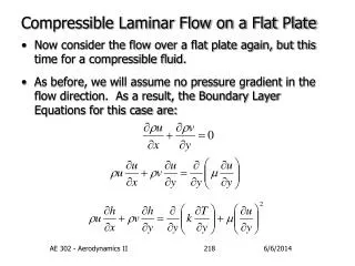
1. Compressible Laminar Flow on a Flat Plate • Now consider the flow over a flat plate again, but this time for a compressible fluid. • As before, we will assume no pressure gradient in the flow direction. As a result, the Boundary Layer Equations for this case are: AE 302 - Aerodynamics II

2. Compressible Laminar Flow [2] • An important modification is to switch to a form of the energy equation in terms of the total enthalpy rather than the local enthalpy. • For a flat plate with near zero vertical velocity, this can be approximated by: • To get this new form, first multiply the x momentum equation by the horizontal velocity. The result is: • Next, add this equation to the existing energy equation. After combining terms this becomes: AE 302 - Aerodynamics II

3. Compressible Laminar Flow [3] • This equation can be simplified on the left-hand-side using the definition of total enthalpy. • The right hand terms can be simplified with some substitutions. First, assuming a thermally perfect gas: • Thus, the heat conduction term can be re-written as: AE 302 - Aerodynamics II

4. Compressible Laminar Flow [4] • The other two terms can be combined using the rules of differentiation by parts: • Put together, these manipulations yield: • From this equation, we can begin to see the importance of the Prandlt number. • In a boundary layer there are competing energy fluxes: • A downward flux due to work done by friction. • An upward flux due to higher temperatures near the wall. AE 302 - Aerodynamics II

5. flux of thermal energy y y flux of work energy T u Compressible Laminar Flow [5] • These two fluxes are represented in the energy equation by the term: • When the Prandlt number is equal to 1.0, these fluxes are in opposing balance – i.e. there is no net flux. • For an adiabatic wall, this means that for Pr = 1: AE 302 - Aerodynamics II

6. Compressible Laminar Flow [6] • For this case, we can also define the adiabatic wall enthalpy and temperature as: • If the Prandlt number is less then one (like in gasses), the flux due to conduction dominates. • In this case the actually wall temperature, even when adiabatic, is less than would be expected: • This “loss” in energy, actually just a redistribution of energy in the flow, can be expressed by a recovery factor, r, define by: AE 302 - Aerodynamics II

7. Van Driest’s Solution • Now, consider a solution to this problem. • The Blassius solution proved the utility of the concept of flow self similarity and transformations. • However, for compressible flow, the application of these concepts is considerably more difficult. • We will discuss the solution first proposed by van Driest using the coordinate transformations: • The x-coordinate transformation only differs by a constant factor from before – but the y-coordinate now includes a factor accounting for the density variation. AE 302 - Aerodynamics II

8. Van Driest’s Solution [2] • The functions of interest , two rather than one, represent the velocity and enthalpy profiles: • Without going into details, the result of this transformation is the two ODE’s: AE 302 - Aerodynamics II

9. Van Driest’s Solution [3] • The boundary conditions which go with these equations are: • Note that these two equations are coupled to each other through the ratio of terms which depends upon temperature. • Since the pressure is still assumed constant through the boundary layer, the density ratio can be written as: • Note this implies a lower density in the BL where the temperature is high. AE 302 - Aerodynamics II

10. Van Driest’s Solution [4] • The viscosities can be found using an empirical approximation known as Sutherland’s Formula: • Using this, the ratio of viscosities is: • With these, and a representation of how Pr and cp vary with temperature and the previous ODE’s can be solved numerically using a coupled, iterative procedure. AE 302 - Aerodynamics II

11. Van Driest’s Solution [5] • In van Driest’s original paper, he assumed a calorically perfect gas and that the Prandlt number is a constant equal to 0.75. • In this case, the remaining group of constants in the equations can be expressed as a function of the external flow Mach number: • The solution for different Mach numbers, while not very difficult to obtain, are tricky due to a poor convergence. • We will concentrate on the solutions, copied from van Driest, presented in the textbook on pages 815-819. AE 302 - Aerodynamics II

12. Adiabatic Wall Solutions • These solutions of BL velocity and temperature profiles are for freestream Mach numbers from 0 to 20. • The things that stick out are the very high temperatures at high M – and the corresponding large BL thickness. • The two factors are related – the high T’s produce low densities which cause the BL to be thicker. • Note that the temperatures are not as high as might be expected. For M=20, the total temperature ratio is: • But, the chart shows a maximum value of around 70. The difference is due to the Prandlt number of 0.75. AE 302 - Aerodynamics II

13. Adiabatic Wall Solutions [2] AE 302 - Aerodynamics II

14. Adiabatic Wall Solutions [3] • In fact, it is not too difficult to show for this case that the recovery factor is given by: • While the recovery factor is less than 1, the temperatures are still extremely high. • The impact this has on BL thickness leads to the observation that was made for hypersonic flow, namely: • This thickened BL will have the effect of decreasing the wall skin friction since the gradients at the wall will be smaller. AE 302 - Aerodynamics II

15. Fixed Wall Temperature Solutions • In the adiabatic wall solutions, the temperature gradient goes to zero at the wall to satisfy the BC there. • The other possibility is to imposed a fixed wall temperature and let the temperature gradient, and thus heat flux, be part of the solution. • Van Driest’s solutions for a cool wall, Tw=0, are given in Figs. 18.6 and 18.7. • Note that the BL thickness is much less than the adiabatic wall due to the lower T’s and higher densities. • The maximum temperatures occur fairly deep inside the BL, but are considerably lower than the adiabatic case. AE 302 - Aerodynamics II

16. Fixed Wall Temperature Solutions [2] AE 302 - Aerodynamics II

17. Compressible Correlations • From the solutions obtained from this solutions method, some correlations for BL thickness and wall skin friction and heat transfer can be made. • These correlations are written in terms of a compressibility correction to the Blassius results. • The correction factors depend upon the flow Mach number, Prandlt number, and wall to edge temperature ratio as follows: • Plots of these correlation functions are given in Figs. 18.8 and 18.9. AE 302 - Aerodynamics II

18. Compressible Correlations [2] AE 302 - Aerodynamics II

19. Compressible Correlations [3] • Note that the skin friction correlation can be made to either the local value or the integrated drag results: • And also note that the thicker the BL, the lower the drag as indicated by the relative corrections for an adiabatic and cool wall. • For the heat transfer to a cool wall, we introduce a new factor, which could be called the heat transfer coefficient, but is properly named the Stanton number: AE 302 - Aerodynamics II

20. Compressible Correlations [4] • In evaluating this property for van Driest’s solutions, it is noted that the value of CH is closely tied to that of cf. • This occurs frequently in heat transfer problems and is due to the very similar natures of viscosity and heat conduction in gasses. • The relationship between the two factors is known as the Reynold’s Analogy and for this case it can be written as: • As a result, the observations made for the skin friction also apply to the heat transfer coefficient. AE 302 - Aerodynamics II

21. Reference Temperature Method • The previous method of van Driest provides an approximate model which gives good insight into the behaviour of compressible boundary layers. • However, the model can be rather complex to solve and the results are still only an approximation. • A simplier method which provides results of comparable accuracy is called the Reference Temperature Method. • In this method, the incompressible results of Blassius are “corrected” for temperature effects observed in a compressible BL. • In particular, the flow properties are evaluated at a reference temperature which depends upon the freestream Mach number and wall temperature. AE 302 - Aerodynamics II

22. Reference Temperature Method [2] • The proposed equation for this reference temperature, T*, in air is: • The surface skin friction coefficient is then given by: • And the Stanton number, using Reynolds analogy, is given by: AE 302 - Aerodynamics II

23. Stagnation Point Heating • Finally, before finishing with laminar flow, consider the situation of a blunt body and the heating which occurs at the stagnation point. • Somewhat surprisingly, the boundary layer at a stagnation point is not infinitely thin, but actually has finite thickness. • In any event, if the wall is non-adiabatic, there will be a thermal boundary layer which needs to be analyzed. • Van Driest also derived the first solutions for this problem using similar methods to that for the flat plate. • The major difference is the fact that the conditions at the edge of the boundary layer are no longer constants. AE 302 - Aerodynamics II

24. Stagnation Point Heating [2] • The coordinate transformations, particularly in the x-direction which now runs along the surface, accounts for this: • The functions are similar, but van Driest did not use the transformation to total enthalpy for this case. • The resulting momentum and energy equations are: AE 302 - Aerodynamics II

25. Stagnation Point Heating [3] • Without proof, a numerical solution to this flow shows that the heat transfer on a cylindrical body is given by: • For a spherical body, a similar, axisymmetric solution gives: • Note that the heat transfer is for the sphere is higher due to the 3-D relaxation effect which leads to a thinner BL and thus higher temperature gradients. • For both cases, however, the heading rate depends upon the gradient in velocity: AE 302 - Aerodynamics II

26. Stagnation Point Heating [4] • For a blunt body, the values of the edge properties can be found from a coupled inviscid flow solution. • The velocity gradient itself can be found using Euler’s equation and the definition of the pressure coefficient: • Combined, these give: • Now, assume that the Mach number is very high so that we can apply our Newtonian flow theory. AE 302 - Aerodynamics II

27. ue R Dx M  Stagnation Point Heating [5] • Thus, the derivative of the pressure gradient is: • Near the stagnation point of a cylinder, using small angle approximations… • Thus: AE 302 - Aerodynamics II

28. Stagnation Point Heating [6] • Similarly, the velocity near the stagnation point can be represented by the first term in a Taylor series: • Combining these, the velocity near the stagnation point can be written as: • So that: • And, thus, the heating rate is inversely proportional the square root of body radius: AE 302 - Aerodynamics II

29. Stagnation Point Heating [7] • This result provides the reasoning behind the blunt design of so many hypersonic vehicles. • Also, you will observe that on some vehicles, like the space shuttle, the curved surfaces like the nose cone and wing leading edge use materials with higher heat tolerance than in other, flatter locations. AE 302 - Aerodynamics II