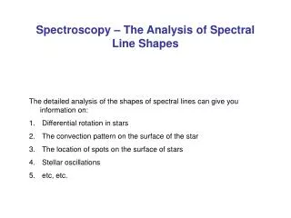
Spectroscopy – The Analysis of Spectral Line Shapes

1. Spectroscopy – The Analysis of Spectral Line Shapes • The detailed analysis of the shapes of spectral lines can give you information on: • Differential rotation in stars • The convection pattern on the surface of the star • The location of spots on the surface of stars • Stellar oscillations • etc, etc.

2. Basic tools for line shape analysis: • The Fourier transform • Line bisectors Both pioneered by David Gray • To derive reliable information about the line shapes requires high resolution and high signal-to-noise ratios: • R = l/dl ≥ 100.000 • S/N > 200-300

3. ∞ ∫ i(f) = I(l)e2pilf dl –∞ Fourier Transform of the Rotation Profile David Gray pioneered using the Fourier transform of spectral lines to derive information from the shapes. Where I(l) is the intensity profile (absorption line) and frequency f is in units of cycles/Å or cycles/pixel (detector units) Because of the inverse relationship between normal and Fourier space (narrow lines translates into wide features in the Fourier domain), the Fourier transform is a sensitive measure of subtle shapes in the line profile. It is also good for measuring rotation profiles.

4. A real spectrograph The Instrumental Profile The observed profile is the spectral line profile of the star convolved with the instrumental profile of the spectrogaph, i(l) What is an instrumental profile (IP)?: Consider a monochromatic beam of light (delta function) Perfect spectrograph

5. No problem with this IP Problems for line shape measurements If the IP of the instrument is asymmetric, then this can seriously alter the shape of the observed line profile It is important to measure the IP of an instrument if you are making line shape measurements

6. If D(Dl) is the observed profile (your data) then D(Dl) = H(Dl)*G(Dl)*I(Dl) • Where: • D = observed data • H = intrinsic spectral line • G = Broadening function (rotation * macroturbulence) • I = Instrumental profile • * = convolution In Fourier space: d(s) = h(s)g(s)i(s) You can either include the instrumental response, I, in the modeling, or deconvolve it from the observed profile.

7. Fourier Transform of the Rotation Profile

8. Fourier Transform of the Rotation Profile The Fourier transform of the rotational profile has zeros which move to lower frequencies as the rotation rate increases (i.e. wider profile in wavelength coordinates means narrower profile in frequency space).

9. Limb Darkening Limb darkening shifts the zero to higher frequency

10. Limb Darkening The limb of the star is darker so these contribute less to the observed profile. You thus see more of regions of the star that have slower rotation rate. So the spectral line should look like a more slowly rotating star, thus the first zero of the transform should move to lower frequencies

11. Limb Darkening Ic/Ic0 = (1 – e) + e cosq

12. Effects of Differential Rotation on Line shapes The sun differentially rotates with equatorial acceleration. The equator rotational period is about 24 days, for the pole it is about 30 days. Differential rotation can be quantified by: w = w0 + w2 sin2f + w4sin4f f is the latitude a= w2/(w0 + w2) Differential rotation parameter Solar case a = 0.19 + → equator rotates faster – → pole rotates faster

13. Effects of Differential Rotation on Line shapes

14. Effects of Differential Rotation on Line shapes

15. The inclination of the star has an effect on the Fourier transform of the differential profile

16. Differential Rotation in A stars In 1977 Gray looked for differential rotation in a sample of A-type star and found none. This is not surprising since we think that the presence of a convection zone is needed for DR and A-type stars have a radiative envelope.

17. Differential Rotation in A stars Gray found two strange stars. g Boo has a weak first sidelobe and no second side lobe. g Her has no sidelobes at all. This may be the effects of stellar pulsations.

18. Differential Rotation in F stars In 1982 Gray looked for differential rotation in a sample of F-type star and concluded that there was no differential rotation. Spot activity on F-type stars is not seen, but they do have a convection zone so DR is possible.

19. Differential Rotation in F stars y Cap a = 0 a = 0.25 However, in 2003 Reiners et al. found evidence for differential rotation in F-stars

20. Velocity Fields in Stars Early on it was realized that the observed shapes of spectral lines indicated a velocity broadening in the photosphere termed „turbulence“ by Rosseland. A theoretical line profile with thermal broadening alone will not reproduce the observed spectral line profile. This macroturbulent velocity broadening is direct evidence of convective motions in the photospheres of stars

21. 1 p½v0 v0cos q b = Dl = cos q l l Dl 2 1 c c ) –( [ exp [ N(Dl)dl = b p½b Dl 2 ) –( [ [ b0cosq From Velocity to Spectrum dv N(v)dv = e–(v/v0)2 N(v)dv is the fraction of material having velocities in the range v → v + dv and v is allowed only on stellar radii. The projection of velocities along the line of sight cos q = b0 1 = dDl exp p½b0cosq Note that b, the width parameter, is a function of q, b0 is constant. At disk center N(l) reflects N(v) directly, but way from the center the Doppler distribution becomes narrower. At the limb N(Dl) is a delta function.

22. Including Macroturbulence in Spectra The observed spectra (ignoring other broadening mechanisms for now) is the intensity profile convolved with the macroturbulent profile: In = In0 * Q(Dl) In0is the unbroadened profile and Q(Dl) is the macroturbulent velocity distribution. What do we use for Q?

23. The Radial-Tangential Prescription from Gray We could just use a Gaussian distribution of radial components of the velocity field (up and down motion), but this is not realistic: Horizontal motion to lane Convection zone Rising hot material Cool, sinking intergranule lane If you included only a distribution of up and down velocities, at the limb these would not alter the line profile at the limb since the motion would not be in the radial direction. The horizontal motion would contribute at the limb Radial motion at disk center → main contrbution at disk center Tangential motion at disk center → main contribution at limb

24. AR AT –(Dl/zTcos q)2 e p½zRcos q p½zTcos q p/2 p/2 ∫ ∫ 2pAT 2pAR QT(Dl)*Insin q cosq dq QR(Dl)*Insin q cosq dq + 0 0 The Radial-Tangential Prescription from Gray Assume that a certain fraction of the stellar surface, AT, has tangential motion, and the rest, AR, radial motion Q(Dl) = ARQR(Dl) + ATQT(Dl) –(Dl/zRcos q)2 e = + And the observed flux Fn=

25. The Radial-Tangential Prescription from Gray The R-T prescription produces as slightly different velocity distribution than an isotropic Gaussian. If you want to get more sophisticated you can include temperature differences between the radial and tangential flows.

26. The Effects of Macroturbulence Macro 10 km/s 5 km/s 2.5 km/s 0 km/s Relative Intensity Pixel shift (1 pixel = 0.015 Å)

27. Macroturbulence versus Luminosity Class Macroturbulence increases with luminosity class (decreasing surface gravity)

28. The Effects of Macroturbulence Relative Flux Amplitude Pixel (0.015 Å/pixel) Frequency (c/Å) There is a trade off between rotation and macroturbulent velocities. You can compensate a decrease in rotation by increasing the macroturbulent velocity. At low rotational velocities it is difficult to distinguish the two. Above the red line represents V = 3 km/s, M = 0 km/s. The blue line represents V=0 km/s, and M = 3 km/s. In wavelength space (left) the differences are barely noticeable. In Fourier space (right), the differences are larger.

29. The Effects of Macroturbulence Rotation affects the location of the first zero. Macroturbulence affects the size of the first side lobe and to a lesser extent the main lobe.

30. m sin i = 11 MJup Most likely vsini is 0-1 km/s. HD 114762 is an F8 star and the mean rotation of these stars is about 5 km/s. The companion could be a more massive companion, maybe even a late M-dwarf Sometimes it is very important to measure the rotational velocity accurately. HD 114762

31. If you want to calculate the Fourier transform of the line you have to „cut out“ the line. This is the equivalent of multiplying your data with a box function. A word of caution about using Fourier transforms In Fourier space this is a sinc function which gets convolved with your broadening function. This changes the FT. → need to apply taper function (bell cosine, etc.)

32. A clue may be found in the slow projected rotational velocity of Vega, an A0 V star The Funny Shape of the Lines of Vega

33. Recall Gravity darkening Teff = C g0.25 ,C is a constant Von Zeipel law (1924): equator Because of gravity darkening and centrifugal force, the equator has lower gravity and a lower temperature. For a star viewed pole on this appears at the limb. Temperature/gravity sensitive weak lines will be stronger at the equator (limb) than at the poles. Rotation pole

34. Span The Power of Spectral Line Bisectors What is a bisector? Curvature

35. Bisectors as a Measure of Granulation Hot rising cell Cool sinking lane

36. Solar Bisector Solar bisectors take on a „C“ shape due to more flux and more area of rising part of convective cells. There is considerable variations with limb angle due to the change of depth of formation and the view angle. The line profiles themselves become shallower and wider towards the limb.

37. Bisectors as a Measure of Granulation The measurement of an individual bisector is very noisy. One should use many lines. These can be from different line strengths as one can „collapse“ them all into one grand mean. Note: this cannot be done in hotter stars the weak lines do not mimic the shape of the top portion of the bisector.

38. Changes in the Granulation Pattern of Dwarfs

39. Changes in the Granulation Supergiants

40. The Granulation and Rotation Boundary Rapid rotation, Inverse „C“ bisectors Slow rotation „C“ shaped bisectors

41. Bisectors as a Measure of Granulation • Can get good results using a 4 stream model (Dravins 1989, A&A, 228, 218). These best reproduce hydrodynamic simulations • Granule center (rising material) • Granules (rising material) • Neutral areas (zero velocity) • Intergranule lanes (cool sinking material) Each has their own fractional areas An, velocity Vn, and Temperature Tn • Constraints: • A1 + A2 + A3 + A4 = 1 • V3 = 0 • Mass conservation: A1×V1 + A2 ×V2 = A4×V4 • Downflow = upflow Best way, is to use numerical hydrodynamic simulations

42. Bisectors as a Measure of Granulation Examples of 4 component fits for stars from Dravins (1989)

43. Rotation amplifies the Bisector span (Gray 1986):

44. Using Bisectors to Study Variability The Effects of Stellar Pulsations

45. Variations of Bisectors with Pulsations

46. The 51 Peg Controversy Gray reported bisector variations of 51 Peg with the same period as the planet. Gray & Hatzes modeled these with nonradial pulsations Gray & Hatzes A beautiful paper that was completely wrong.

47. Hatzes et al. More and better bisector data for 51 Peg showed that the Gray measurements were probably wrong. 51 Peg has a planet!

48. Bisector Variations due to Spots Spot Pattern Changes in Radial Velocity due to changing shapes

49. Star Patches Bisectors Bisector span

50. Star Patches DT = 300 K Compared to DT = 2000 K for sunspots