Download
1 / 24
240 likes | 426 Vues
Epistasis Genome-wide association interaction analysis (GWAI). Elena S. Gusareva, PhD egusareva@ulg.ac.be (1) Systems and Modeling Unit, Montefiore Institute (2) Bioinformatics and Modeling , GIGA-R Université de Liège Belgium. Outline.

E N D
Epistasis Genome-wide association interaction analysis (GWAI) Elena S. Gusareva, PhD egusareva@ulg.ac.be (1) Systems and Modeling Unit, Montefiore Institute (2) Bioinformatics and Modeling, GIGA-R Université de Liège Belgium
Outline • Epistasis: definition and example of biological epistasis • Protocol for genome-wide association interaction analysis (GWAI) • Data collection • Quality control • Choosing a strategy for GWAI (exhaustive and selective epistasis screening) • Tests of association • LD-pruning • Confounders and population stratification • Interpretation and follow-up (replication analysis and validation) • GWAI screening: an example on Alzheimer’s disease
Human diseases Monogenic disease - Phenylketonuria (Phenylalanine hydroxylase – PAH gene) mutation Linkage analysis Complex disease - Crohn's disease (99 disease susceptibility loci ~ 25% of heritability of CD) MISSING HERITABILITY !!! GWA analysis
Missing heritability • Where does heritability hide? • Overestimated heritability • Inaccurate definition of pathological traits • Low frequency variants and rare variants • De novo mutations • Epigenetic effects, CNVs, STRs, etc. • Gene X Environment interactions effects • Epistasis • Etc.
Biological epistasis • William Bateson, 1909 - “compositional epistasis” driven by biology • Distortions of Mendelian segregation ratios due to one gene masking the effects of another • Whenever two or more loci interact to create new phenotypes • Whenever an allele at one locus masks or modifies the effects of alleles at one or more other loci Epistasis is an interaction at the phenotypic level of organization. It does not necessary imply biochemical interaction between gene products. How blue eyed parents can have a brown eyed child? By Dr. Barry Starr, Stanford University
Simple examples of epistasis Genes interact to create new phenotypes Anthocyanin pigment compound for pea flower Gene 2: p/P - white Gene 1: c/C - white precursor Step 1 Step 2 purple Masking effect of gene Gene 2: g/G - dominant Hair color in mice Gene 1: BB and bB – black bb - white X grey
Statistical epistasis Ronald Fisher, 1918 - “statistical epistasis” Epistasis is when two (or more) different genes contribute to a single phenotype and their effects are not merely additive (deviations from a model of additive multiple effects for quantitative traits). ÖrjanCarlborg and Chris S. Haley, Nature Reviews Genetics, V 5, 2004
Why is there epistasis? • C.H. Waddington, 1942: canalization and stabilizing selection theory: • Phenotypes are stable in the presence of mutations through natural selection. • The genetic architecture of phenotypes is comprised of networks of genes that are redundant and robust. • Only when there are multiple mutational hits to the gene network occur the phenotypes can change dramatically. • Epistasis create dependencies among the genes in the network and thus keep the stability of the system. Identification of epistasis is a step to systems-level genetics where we can understand all the complexity of underling biology of the complex traits. Greenspan, R. The flexible genome. Nature Reviews Genetics 2,385.
How big can be a disease variance due to epistasis? Joshua S. Bloom et al. & Leonid Kruglyak, Nature 2013 Finding the sources of missing heritability in a yeast cross. Researchers mated two yeast strains (BY from a laboratory and RM from a vineyard) and collected the offspring (tetrads) for genome-wide analysis to look for gene variations that contributed to survival (46 quantitative traits). This experimental setup allowed the researchers to determine how much of the inherited survival traits could be detected by genome-wide scan and how much was "missing" or undetectable using a genome-wide scan. (Illustration by Joshua Bloom, Kruglyak Lab) • Broad-sense heritability (total heritability) - narrow-sense heritability (heritability due to main-effect variants or additive genetic factors) = variance due to gene–gene interactions: • from 2% to 54% of heritability • from 1 till 16 pair-wise interactions associated with 24 quantitative traits • two-locus interactions in which neither locus has a detectable main effect were uncommon
Complications in humans • ??? Can we use the statistical evidence of epistasis at the population level to infer biological or genetical epistasis in an individual? • ??? Does biological evidence of epistasis imply that statistical evidence will be found? • Epistasis can be very complex depending on • Number of loci in epistasis (if more than one epistatic interaction occurs to cause a disease, then identifying the genes involved and defining their relationships becomes even more difficult.) • Manner of inheritance of each particular locus (dominant, co-dominant, recessive, additive) • Gene penetrance • Confounding factors: environment, age, gender, etc. • The trait (phenotype) they contribute to (binary, continuous, complex traits - disease)
Ho to identify epistasis? There are plenty methods exist each utilizing different statistical methodologies and addressing different aspects of biological epistais. Kilpatrick 2009 Clear strategy is required…
Protocol for GWAI • 0. Data collecting and genotyping 1. Samples and markers quality control (e.g. SVS 7.5, PLINK software): HWE test (P >1*10-4), call rate > 98%, marker allele frequency (MAF > 0.05) Exhaustive epistasis screening (a) Selective epistasis screening (b) 2.b.1 Selection ofSNPs basing on their function (e.g. SNPper - SNP Finder tool) 2.b.1 Selection ofSNPs from candidate genes (data from literature) 2.b.1 Markers prioritization/pre-filtering (e.g. Biofilter 1.1.0 tool) 2.a.1 LD pruning (e.g. SVS 7.5, PLINK software): window size 50 bp, window increment 1 bp, LD r2threshold 0.75 2.b.2 LD pruning (e.g. SVS 7.5, PLINK software): window size 50 bp, window increment 1 bp, LD r2 threshold 0.75 2.a.3 Exhaustive genome-wide screening for pair-wise SNP interactions (e.g. BOOST analysis) 2.b.3 Adjustment for confounders (e.g. R software, via logistic regression), family structure (e.g. GenABEL software, via mixed polygenic model), population stratification (e.g. GenABEL software, via mixed polygenic model; SVS 7.5 software, via PCA) 2.b.4 (Genome-Wide) Screening for pair-wise SNP interactions (e.g. MB-MDR2D analysis, SD plot, logistic regression-based methods) 3. Replication analysis with alternative methods for epistasis detection: follow up the selected set of markers (e.g. MB-MDR2D analysis, SD plot, logistic regression-based methods) 4. Replication of epistasis in the independent data and meta-analysis (e.g. fixed effects and random effects models) 5. Biological validation (e.g. immunological pathway analysis, eQTL analysis, DNA transcription factor binding sites analysis, composite elements binding sites analysis, etc.)
Selecting strategy for GWAI • The exhaustive screening includes testing for all possible pair-wise interactions across all genetic markers. • + all information is used for the analysis • + new genetic loci can be detected • - computationally demanding • - test statistics has to be quite simple to be run in a reasonable time • - power the analysis has to be very large to pass through stringent multiple testing criteria • The selective screening, exploits particular assumptions and/or special methods to substantially reduce number of markers in the analysis and search for pair-wise interactions only across potentially more promising genetic loci. • + computationally less demanding • + more robust statistical methods can be applied (including adjustment for confounders) • + less severe multiple testing correction is needed • - smaller chance for detection of previously unreported epistasis
Pre-filtering of genetic markers for selective screening • The selection of genetic markers is usually based on prior expert knowledge about a trait/disease under investigation. • candidate genes/markers • markers from coding regions of genes that can potentially change protein structure • selection using filtering tools that take into account the biology behind the trait under investigation • Biofilteruses biological information about gene-gene relationships and gene-disease relationships to construct multi-SNP models before conducting any statistical analysis. Model production is gene centric. • Biofilter data-sources: • Gene Ontology • KEGG - The Kyoto Encyclopedia of Genes and Genomes • Net Path - source of curated immune signaling and cancer pathways • PFAM - Protein Families Database • Reactome- database of curated core pathways and reactions in human biology • DIP - The Database of Interacting Proteins
Exhaustive epistasis screening method • BOOST (BOolean Operation-based Screening and Testing) is a fast two-stage (screening and testing) approach to search for epistasis associated with a binary outcome. • Stage 1: In the screening stage, a non-iterative method is used to approximate the likelihood ratio statistic. • Stage 2: In the testing stage, the classical likelihood ratio test is employed to measure the interaction effects of selected SNP pairs • + can calculated interaction around over 0.5 millions of SNPs • - can not deal with continuous traits (only for binary traits) • cannot deal with LD • does not perform automatically the multiple testing correction • has limitations with respect to statistical power • The BOOST is based on simple logistic regression (co-dominant model of inheritance): A logistic regression produces a logistic curve, which is limited to values between 0 and 1. Logistic regression is similar to a linear regression, but the curve is constructed using the natural logarithm of the “odds” of the independent variable, rather than the probability. Moreover, the predictors do not have to be normally distributed or have equal variance in each group.
Selective epistasis screening methods: MB-MDR Model-Based Multifactor Dimensionality Reduction (MB-MDR) method implies association testing between a trait and a factor consisting of multilocus genotype information. Step1: For every pair of markers, each multilocus genotype (MLG) is tested for association with a trait against of the group of other MLGs. Basing on this statistics each MLG is classified as “high risk”, “low risk” or “no evidence for risk” (by default risk threshold = 0.1), and than all MLGs of the same class are merged. Step2: For each risk category, “high” and “low” (captures summarized information about the importance of the pair of markers), a new association test is performed. Step3: The significance is explored through a permutation test (1000 permutations) and correction for the multiple testing H L vs + binary and continuous traits + different study designs + adjustment for covariates + adjust for main effect - computationally demanding
Selective epistasis screening methods: SD plot Synergy disequilibrium (SD) method: to assess interaction in a small set of genetic markers and graphically represent the results The synergy between two SNPs Siand Sjwith respect to a trait/disease C is defined as the amount of information conveyed by the pair of SNPs about the presence of the disease, minus the sum of the corresponding amounts of information conveyed by each SNP: I(Si,Sj;C)−[I(Si;C)+I(Sj;C)] • + can distinguish between LD and epistasis • + good for results visualization • does not correct for multiple testing • can be used for a limited number of markers
Marker LD pruning • LD pruning is a procedure of filtering genetic markers by linkage disequilibrium leaving for the analysis only tagging SNPs that are representatives of the genetic haplotype blocks. • + allow avoiding top ranked SNP-SNP interactions that are redundant and merely due to the high correlation between genetic markers. • + decrease computational burden • + relax the excessive multiple testing correction • LD, correlation between SNPs, is calculated via r2 statistics - Pearson test statistic for independence in a 2 × 2 table of haplotype counts. • LD r2filtering threshold > 0.75 (rather conservative but will best minimize the amount of redundant interactions). • LD pruning procedure in SVS (Golden Helix Inc.) • For any pair of markers under testing whose r2 > 0.75, the first marker of the pair is discarded. • Window increment 1 (number of markers by which the beginning window position was incremented). Where pi, pjare the marginal allelic frequencies at the ithand jthSNP respectively and pijis the frequency of the two-marker haplotype
Confounding factors in genetic studies A variable can confound the results of a statistical analysis only if it is related to both the dependent variable and at least one of the other independent variables in the analysis and also do not lie in the directed causal path from the dependent to independent variable. Special case of confounding factors: Population stratification is a systematic difference in allele frequencies between subpopulations in a population. The basic cause of population stratification is different genetic ancestry as a result of nonrandom mating between subgroups in a population due to various reasons (social, cultural, geographical, etc.). The shared ancestry corresponds to relatedness, or kinship, and so population structure can be defined in terms of patterns of kinship among groups of individuals. Independent variable – Cause (e.g. genetic factors) Dependent variable – Effect (e.g. disease trait) Confounding variable (e.g. sex, age, genetic background, ethnicity, etc.)
Principal component analysis (PCS) What is PCA? It is a way of identifying patterns in data, and expressing the data in such a way as to highlight their similarities and differences. PCA allows data transformation to a new coordinate system such that the projection of the data along the first new coordinate has the largest variance; the second principal component has the second largest variance, and so on. + easy to apply + availability of efficient algorithms + easy to adjust variables for by including PCs in regression models - not clear how to select an optimal number of PCs for adjustment - change the original presentation of the variables (specially severe for binary traits) - does not take care of cryptic relatedness (when apparently unrelated individuals actually have some unsuspected relatedness )
Protocol for GWAI • 0. Data collecting and genotyping 1. Samples and markers quality control (e.g. SVS 7.5, PLINK software): HWE test (P >1*10-4), call rate > 98%, marker allele frequency (MAF > 0.05) Exhaustive epistasis screening (a) Selective epistasis screening (b) 2.b.1 Selection ofSNPs basing on their function (e.g. SNPper - SNP Finder tool) 2.b.1 Selection ofSNPs from candidate genes (data from literature) 2.b.1 Markers prioritization/pre-filtering (e.g. Biofilter 1.1.0 tool) 2.a.1 LD pruning (e.g. SVS 7.5, PLINK software): window size 50 bp, window increment 1 bp, LD r2threshold 0.75 2.b.2 LD pruning (e.g. SVS 7.5, PLINK software): window size 50 bp, window increment 1 bp, LD r2 threshold 0.75 2.a.3 Exhaustive genome-wide screening for pair-wise SNP interactions (e.g. BOOST analysis) 2.b.3 Adjustment for confounders (e.g. R software, via logistic regression), family structure (e.g. GenABEL software, via mixed polygenic model), population stratification (e.g. GenABEL software, via mixed polygenic model; SVS 7.5 software, via PCA) 2.b.4 (Genome-Wide) Screening for pair-wise SNP interactions (e.g. MB-MDR2D analysis, SD plot, logistic regression-based methods) 3. Replication analysis with alternative methods for epistasis detection: follow up the selected set of markers (e.g. MB-MDR2D analysis, SD plot, logistic regression-based methods) 4. Replication of epistasis in the independent data and meta-analysis (e.g. fixed effects and random effects models) 5. Biological validation (e.g. immunological pathway analysis, eQTL analysis, DNA transcription factor binding sites analysis, composite elements binding sites analysis, etc.)
Epistasis replication and validation Given the availability of a comprehensive meta-analysis toolbox, it may be surprising that hardly any meta-GWAIs have been published as the core topic of the publication. (Mission Impossible @ google) Original study Random variation • Validation: • Gene-based rather then genetic • variants-based validation analysis • Meta-analytic approaches (replication analysis in an independent sample) • Trustworthy biological validation (systematic literature review, use of structured knowledge from databases, biological experiments) samples Original population Different population Systematic variation samples samples Replication study Validation Igl et al. 2009
Biological validation of statistical epistasis signals J Thornton, EBI
Useful public sources for studding biology behind statistical epistais signals http://www.ncbi.nlm.nih.gov/ - The National Center for Biotechnology Information (NCBI) advances science and health by providing access to biomedical and genomic information. http://www.ensembl.org/index.html – The Ensemblproject produces genome databases for vertebrates and other eukaryotic species, and makes this information freely available online. http://hapmap.ncbi.nlm.nih.gov/ – HapMap– multi-country effort to identify and catalog genetic similarities and differences in human beings. http://lynx.ci.uchicago.edu/ - LYNX – Gene Annotations, Enrichment Analysis and Genes Prioritization. http://www.genemania.org/– GeneMANIA- Indexing 1,421 association networks containing 266,984,699 interactions mapped to 155,238 genes from 7 organisms.