Download
1 / 6
60 likes | 123 Vues
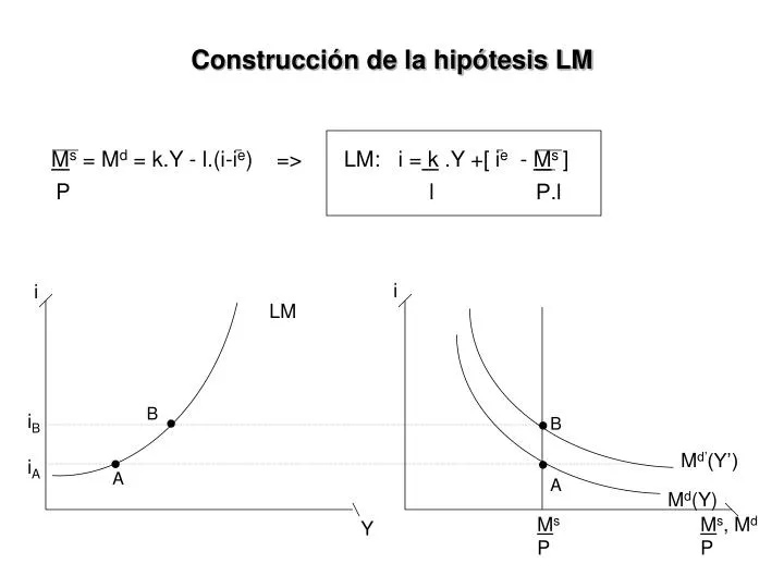
Construcción de la hipótesis LM. M s = M d = k.Y - l.(i-i e ) => LM: i = k .Y +[ i e - M s ] P l P.l. i. i. LM. B. i B. B. M d’ (Y’). i A. A. A. M d (Y). Y. M s P. M s , M d P. Trampa de Liquidez.

E N D
Construcción de la hipótesis LM Ms = Md = k.Y - l.(i-ie) => LM: i = k .Y +[ ie - Ms ] P l P.l i i LM . . B iB B . . Md’(Y’) iA A A Md(Y) Y Ms P Ms, Md P
Trampa de Liquidez Md = k.Y - l.(i-ie) Y, Md(Y) , EDM = EOBo, Pb, i, Md(i) k l LM i i . . . A = B i = 0 iA = iB Md(Y1) A B Y1 Y Ms P Ms’ P Ms, Md P
Gambling Casino Grupo 1 “ilíquidos” : C + I 3 grupos de agentes económicos: ● La Crisis del ´30 nuevamente: ● Gran incertidumbre => “l” →∞ => “La Viuda” → EDBo no => Pb, i <=> ante i infinitésima, Md →∞ :los especuladores ofrecen instantáneamente sus bonos: creen que el Pb de hoy se revertirá mañana => venden “caro”. => Ruptura del proceso de intermediación financiera: → el exceso de liquidez en los mercados financieros no se canaliza a (C+I) → pese a poseer fuentes de financimiento, la economía no logra salir de la recesión, queda estancada en una trampa de liquidez. El Gobierno: ¿política monetaria o fiscal? Grupo 2 “líquidos” : mercados financieros El Gobierno
Desequilibrio LM i i LM . . . . D D C C i1 . . . . B i0 B A A Md’ Md Y Ms P Ms, Md P Vía Y Proceso de Ajuste Vía i
Desequilibrio IS - LM i LM I . . I : EOBi, EOM II: EOBi, EDM III: EDBi, EDM IV: EDBi, EOM C C’ IV II . D . . A B IS III Y (A) EDBi Y, Md(Y) (B) EDM EOBo, Pb, i (C) I, DA, Y Md(i) (D)
Velocidad de Ajuste Tiempo lógico vs. Tiempo histórico i i LM LM en el límite ajusta sobre LM . . D D . . A A IS IS Y Y