Download

1 / 55
550 likes | 782 Vues
In The Name Of God Algorithms Design Greedy Algorithms. Dr. Shahriar Bijani Shahed University Feb. 2014. Slides References. Kleinberg and Tardos, Algorithm Design , CSE 5311, M Kumar, Spring 2007. Chapter 4, Computer Algorithms , Horowitz ,…, 2001.

E N D
In The Name Of GodAlgorithms DesignGreedy Algorithms Dr. Shahriar Bijani Shahed University Feb. 2014
Slides References Algorithms Design, Greedy Algorithms Kleinberg and Tardos, Algorithm Design, CSE 5311, M Kumar, Spring 2007. Chapter 4, Computer Algorithms, Horowitz ,…, 2001. Chapter 16, Introduction to Algorithms, CLRS , 2001.
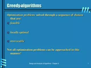
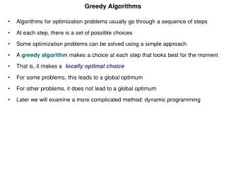
The Greedy Principle • The problem: We are required to find a feasible solution that either maximizes or minimizes a given objective solution. • It is easy to determine a feasible solution but not necessarily an optimal solution. • The greedy method solves this problem in stages, at each stage, a decision is made considering inputs in an order determined by the selection procedure which may be based on an optimization measure. Algorithms Design, Greedy Algorithms
Optimization problems • An optimization problem is one in which you want to find, not just a solution, but the best solution • A “greedy algorithm” sometimes works well for optimization problems • A greedy algorithm works in phases. At each phase: • You take the best you can get right now, without regard for future consequences • You hope that by choosing a local optimum at each step, you will end up at a global optimum Algorithms Design, Greedy Algorithms
Example: Counting money • Suppose you want to count out a certain amount of money, using the fewest possible bills and coins • A greedy algorithm would do this would be:At each step, take the largest possible bill or coin that does not overshoot • Example: To make $6.39, you can choose: • a $5 bill • a $1 bill, to make $6 • a 25¢ coin, to make $6.25 • A 10¢ coin, to make $6.35 • four 1¢ coins, to make $6.39 • For US money, the greedy algorithm always gives the optimum solution Algorithms Design, Greedy Algorithms
A failure of the greedy algorithm • In some (fictional) monetary system, “Rial” come in 1 Rial, 7 Rial, and 10 Rial coins • Using a greedy algorithm to count out 15 Rials, you would get • A 10 Rial piece • Five 1 Rial pieces, for a total of 15 Rials • This requires six coins • A better solution would be to use two 7 Rial pieces and one 1 Rial piece • This only requires three coins • This greedy algorithm results in a solution, but not in an optimal solution Algorithms Design, Greedy Algorithms
You have to run nine jobs, with running times of 3, 5, 6, 10, 11, 14, 15, 18, and 20 minutes You have three processors on which you can run these jobs You decide to do the longest-running jobs first, on whatever processor is available Time to completion: 18 + 11 + 6 = 35 minutes This solution isn’t bad, but we might be able to do better 20 10 3 18 11 6 15 14 5 A scheduling problem P1 P2 P3 Algorithms Design, Greedy Algorithms
What would be the result if you ran the shortest job first? Again, the running times are 3, 5, 6, 10, 11, 14, 15, 18, and 20 minutes That wasn’t such a good idea; time to completion is now 6 + 14 + 20 = 40 minutes Note, however, that the greedy algorithm itself is fast All we had to do at each stage was pick the minimum or maximum 3 10 15 5 11 18 6 14 20 Another approach P1 P2 P3 Algorithms Design, Greedy Algorithms
This solution is clearly optimal (why?) Clearly, there are other optimal solutions (why?) How do we find such a solution? One way: Try all possible assignments of jobs to processors Unfortunately, this approach can take exponential time Better solutions do exist: P1 P2 P3 20 14 18 11 5 15 10 6 3 An optimum solution Algorithms Design, Greedy Algorithms
The Huffman encoding algorithm is a greedy algorithm You always pick the two smallest numbers to combine Average bits/char:0.22*2 + 0.12*3 +0.24*2 + 0.06*4 +0.27*2 + 0.09*4= 2.42 The Huffman algorithm finds an optimal solution 100 54 27 46 15 Huffman encoding A=00B=100C=01D=1010E=11F=1011 2212246279A B C D E F Algorithms Design, Greedy Algorithms
Procedure Huffman_Encoding(S,f); Input : S (a string of characters) and f (an array of frequencies). Output : T (the Huffman tree for S) 1. insert all characters into a heap H according to their frequencies; 2. whileH is not empty do 3. ifH contains only one character xthen 4.x root (T); 5. else 6. z ALLOCATE_NODE(); 7. x left[T,z] EXTRACT_MIN(H); 8. y right[T,z] EXTRACT_MIN(H); 9. fzfx + fy; 10. INSERT(H,z); CSE 5311 Spring 2007 M Kumar
Complexity of Huffman algorithm • Building a heap in step 1 takes O(n) time • Insertions (steps 7 and 8) and • deletions (step 10) on H • take O (log n) time each • ThereforeSteps 2 through 10 take O(n logn) time • Thus the overall complexity of the algorithm is • O( n logn ). CSE 5311 Spring 2007 M Kumar
Knapsack Problem Algorithms Design, Greedy Algorithms Assume a thief is robbing a store with various valued and weighted objects. Her bag can hold only W pounds. The 0-1 knapsack problem: must take all or nothing The fractional knapsack problem: can take all or part of the item
Where Greedy Fails 50 50 50 50 50 20 20 --- 30 30 30 30 20 20 0-1 knapsack 20 10 10 10 10 $60 $120 =$160 $100 =$220 =$180 =$240
Fractional Knapsack Problem • Given n items of sizes w1, w2, …, wn and values p1, p2, …, pn and size of knapsack of C, the problem is to find x1, x2, …, xn that maximize subject to
Solution to Fractional Knapsack Problem • Consider yi= pi / wi • What is yi? • What is the solution? • fractional problem has greedy-choice property, 0-1 does not.
Critical Path Method (CPM) Activity On Edge (AOE) Networks: • Tasks (activities) : a0, a1,… • Events : v0,v1,… V6 V1 a3 = 1 a6 = 9 a9 = 2 a0 = 6 start V0 V4 V8 finish a1 = 4 a10 = 4 a4 = 1 a7 = 7 V7 V2 Some definition: • Predecessor • Successor • Immediate predecessor • Immediate successor a2 = 5 a8 = 4 a5 = 2 V3 V5
CPM: critical path • A critical path is a path that has the longest length. (v0, v1, v4, v7, v8) V6 V1 a3 = 1 a6 = 9 a9 = 2 a0 = 6 start V0 V4 V8 finish a1 = 4 a10 = 4 a4 = 1 a7 = 7 V7 V2 a2 = 5 a8 = 4 6 + 1 + 7 + 4 = 18 (Max) a5 = 2 V3 V5
The earliest time • The earliest time of an activity, ai, can occur is the length of the longest path from the start vertex v0 to ai’s start vertex. (Ex: the earliest time of activity a7 can occur is 7.) • We denote this time as early(i) for activity ai.∴ early(6) = early(7) = 7. V6 V1 a3 = 1 a6 = 9 a9 = 2 a0 = 6 7/? 6/? 0/? 16/? start V0 V4 V8 finish 7/? 14/? a1 = 4 4/? 18 a10 = 4 0/? a4 = 1 a7 = 7 V7 V2 0/? a2 = 5 a8 = 4 7/? a5 = 2 V3 V5 5/?
The latest time • The latest time, late(i), of activity, ai, is defined to be the latest time the activity may start without increasing the project duration. • Ex: early(5) = 5 & late(5) = 8; early(7) = 7 & late(7) = 7 V6 V1 a3 = 1 a6 = 9 a9 = 2 a0 = 6 7/7 6/6 0/0 16/16 start V0 V4 V8 finish 7/7 14/14 a1 = 4 4/5 a10 = 4 0/1 a4 = 1 a7 = 7 V7 V2 0/3 a2 = 5 a8 = 4 7/10 late(5) = 18 – 4 – 4 - 2 = 8 late(7) = 18 – 4 – 7 = 7 a5 = 2 V3 V5 5/8
Critical activity • A critical activity is an activity for which early(i) = late(i). • The difference between late(i) and early(i) is a measure of how critical an activity is. CalculationofEarliest Times FindingCritical path(s) To solveAOE Problem CalculationofLatest Times
Calculation of Earliest Times • Let activity ai is represented by edge (u, v). • early (i) = earliest [u] • late (i) = latest [v] – duration of activity ai • We compute the times in two stages:a forward stage and a backward stage. • The forward stage: • Step 1: earliest [0] = 0 • Step 2: earliest [j] = max {earliest [i] + duration of (i, j)}i is in P(j) P(j) is the set of immediate predecessors of j.
Calculation of Latest Times • The backward stage: • Step 1: latest[n-1] = earliest[n-1] • Step 2: latest [j] = min {latest [i] - duration of (j, i)}i is in S(j) S(j) is the set of vertices adjacent from vertex j. latest[8] = earliest[8] = 18 latest[6] = min{earliest[8] - 2} = 16 latest[7] = min{earliest[8] - 4} = 14 latest[4] = min{earliest[6] – 9; earliest[7] – 7} = 7 latest[1] = min{earliest[4] - 1} = 6 latest[2] = min{earliest[4] - 1} = 6 latest[5] = min{earliest[7] - 4} = 10 latest[3] = min{earliest[5] - 2} = 8 latest[0] = min{earliest[1] – 6; earliest[2] – 4; earliest[3] – 5} = 0
Graph with non-critical activities deleted V6 V1 a9 a0 a3 a6 V8 V0 V4 a1 V2 V7 finish start a4 a7 a10 a2 V3 V5 a8 a5 a6 V6 a9 a0 V1 a3 start V0 V4 V8 finish a7 V7 a10
CPM for the longest path problem • The longest path(critical path) problem can be solved by the critical path method(CPM) : Step 1:Find a topological ordering. Step 2: Find the critical path.
A salesman must visit every city (starting from city A), and wants to cover the least possible distance He can revisit a city (and reuse a road) if necessary He does this by using a greedy algorithm: He goes to the next nearest city from wherever he is From A he goes to B From B he goes to D This is not going to result in a shortest path! The best result he can get now will be ABDBCE, at a cost of 16 An actual least-cost path from A is ADBCE, at a cost of 14 A B C 2 4 3 3 4 4 D E Traveling salesman Algorithms Design, Greedy Algorithms
Analysis • A greedy algorithm typically makes (approximately) n choices for a problem of size n • (The first or last choice may be forced) • Hence the expected running time is:O(n * O(choice(n))), where choice(n) is making a choice among n objects • Counting: Must find largest useable coin from among ksizes of coin (k is a constant), an O(k)=O(1) operation; • Therefore, coin counting is (n) • Huffman: Must sort n values before making n choices • Therefore, Huffman is O(n log n) + O(n) = O(n log n) Algorithms Design, Greedy Algorithms
Single Source Shortest Path • In a shortest-paths problem, we are given a weighted, directed graph G = (V,E), with weights assigned to each edge in the graph. The weight of the path p = (v0, v1, v2, …, vk) is the sum of the weights of its edges: • v0 v1 v2 . . . vk-1 vk • The shortest-path from u to v is given by d(u,v) = min {weight (p)} : if there are one or more paths from u to v = otherwise Algorithms Design, Greedy Algorithms
Dijkstra: Single-Source Shortest Paths Given G (V,E), find the shortest path from a given vertex u V to every vertex v V ( u v). For each vertex v V in the weighted directed graph, d[v] represents the distance from u to v. Initially, d[v] = 0 when u = v. d[v] = if (u,v) is not an edge d[v] = weight of edge (u,v) if (u,v) exists. Dijkstra's Algorithm : At every step of the algorithm, we compute, d[y] = min {d[y], d[x] + w(x,y)}, where x,y V. Dijkstra's algorithm is based on the greedy principle because at every step we pick the path of least weight. Algorithms Design, Greedy Algorithms
Dijkstra's Single-source shortest path Procedure Dijkstra's Single-source shortest path_G(V,E,u) Input: G =(V,E), the weighted directed graph and v the source vertex Output: for each vertex, v, d[v] is the length of the shortest path from u to v. • mark vertex u; • d[u] 0; • for each unmarked vertex vVdo • if edge (u,v) existsd [v] weight (u,v); • else d[v] ; • while there exists an unmarked vertex do • let v be an unmarked vertex such that d[v] is minimal; • mark vertex v; • for all edges (v,x) such that x is unmarked do • if d[x] > d[v] + weight[v,x] then • d[x] d[v] + weight[v,x] Algorithms Design, Greedy Algorithms
Dijkstra's Single-source shortest path Complexity of Dijkstra's algorithm: • Steps 1 and 2 take (1) time • Steps 3 to 5 take O(V) time • The vertices are arranged in a heap in order of their paths from u • Updating the length of a path takes O(log V) time. • There are V iterations, and at most E updates • Therefore the algorithm takes O((E+V) log V) time. Algorithms Design, Greedy Algorithms
6 6 c c c a a a 1 1 1 4 4 2 2 d d d b b 3 b 3 Minimum Spanning Tree (MST) • Spanning tree of a connected graph G: a connected acyclic subgraph of G that includes all of G’s vertices • Minimum spanning tree of a weighted, connected graph G: a spanning tree of G of the minimum total weight • # MST = nn-2 (n = numbers of nodes) Example:
Prim’s MST algorithm • Start with tree T1 consisting of one (any) vertex and “grow” tree one vertex at a time to produce MST through a series of expanding subtrees T1, T2, …, Tn • On each iteration, construct Ti+1 from Ti by adding vertex not in Ti that is closest to those already in Ti (this is a “greedy” step!) • Stop when all vertices are included
4 4 4 4 4 c c c c c a a a a a 1 1 1 1 1 6 6 6 6 6 2 2 2 2 2 d d d d d b b b b b 3 3 3 3 3 Example
Notes about Prim’s algorithm • Proof by induction that this construction actually yields an MST (CLRS, Ch. 23.1). • Efficiency • O(n2)for weight matrix representation of graph and array implementation of priority queue • O(m log n) for adjacency list representation of graph with n vertices and m edges and min-heap implementation of the priority queue
Kruskals_ MST • The algorithm maintains a collection VS of disjoint sets of vertices • Each set W in VS represents a connected set of vertices forming a spanning tree • Initially, each vertex is in a set by itself in VS • Edges are chosen from E in order of increasing cost, we consider each edge (v, w) in turn; v, w V. • If v and w are already in the same set (say W) of VS, we discard the edge • If v and w are in distinct sets W1 and W2 (meaning v and/or w not in T) we merge W1 with W2 and add (v, w) to T.
Kruskal's Algorithm • Procedure MCST_G(V,E) • (Kruskal's Algorithm) • Input: An undirected graph G(V,E) with a cost function c on the edges • Output: T the minimum cost spanning tree for G • T 0; • VS 0; • for each vertex v V do • VS = VS {v}; • sort the edges of E in nondecreasing order of weight • whileVS > 1 do • choose (v,w) an edge E of lowest cost; • delete (v,w) from E; • if v and w are in different sets W1 and W2 in VS do • W1 = W1 W2; • VS = VS - W2; • T T (v,w); • return T
A A 3 3 F 3 1 B 2 F 1 B 2 2 6 4 2 E C 5 E 1 C 1 D D The equivalent Graph and the MCST Kruskals_ MST Consider the example graph shown earlier, The edges in nondecreasing order [(A,D),1],[(C,D),1],[(C,F),2],[(E,F),2],[(A,F),3],[(A,B),3], [(B,E),4],[(D,E),5],[(B,C),6] EdgeActionSets in VS Spanning Tree, T =[{A},{B},{C},{D},{E},{F}]{0}(A,D) merge [{A,D}, {B},{C}, {E}, {F}] {(A,D)} (C,D) merge [{A,C,D}, {B}, {E}, {F}] {(A,D), (C,D)} (C,F) merge[{A,C,D,F},{B},{E}]{(A,D),(C,D), (C,F)} (E,F) merge[{A,C,D,E,F},{B}]{(A,D),(C,D), (C,F),(E,F)}(A,F) reject[{A,C,D,E,F},{B}]{(A,D),(C,D), (C,F), (E,F)}(A,B) merge[{A,B,C,D,E,F}]{(A,D),(A,B),(C,D), (C,F),(E,F)}(B,E) reject(D,E) reject(B,C) reject
Kruskals_ MST Complexity • Steps 1 thru 4 take time O (V) • Step 5 sorts the edges in nondecreasing order in O (E log E ) time • Steps 6 through 13 take O (E) time • The total time for the algorithm is therefore given by O (E log E) • The edges can be maintained in a heap data structure with the property, E[PARENT(i)] E[i] • This property can be used to sort data elements in nonincreasing order. • Construct a heap of the edge weights, the edge with lowest cost is at the root During each step of edge removal, delete the root (minimum element) from the heap and rearrange the heap. • The use of heap data structure reduces the time taken because at every step we are only picking up the minimum or root element rather than sorting the edge weights.
Minimum-Cost Spanning Trees (Application) Consider a network of computers connected through bidirectional links. Each link is associated with a positive cost: the cost of sending a message on each link. This network can be represented by an undirected graph with positive costs on each edge. In bidirectional networks we can assume that the cost of sending a message on a link does not depend on the direction. Suppose we want to broadcast a message to all the computers from an arbitrary computer. The cost of the broadcast is the sum of the costs of links used to forward the message.
Activity Selection Problem • Problem Formulation • Given a set of n activities, S = {a1, a2, ..., an}thatrequire exclusive use of a common resource, find the largest possible set of nonoverlapping activities (also called mutually compatible). • For example, scheduling the use of a classroom. • Assume that aineeds the resource during period [si, fi), which is a half-open interval, where • si = start time of the activity, and • fi = finish time of the activity. • Note: Could have many other objectives: • Schedule room for longest time. • Maximize income rental fees.
Activity Selection Problem: Example • Assume the following set S of activities that are sorted by their finish time, find a maximum-size mutually compatible set.
Solving the Activity Selection Problem • Define Si,j= {akS : fi sk< fksj} • activities that start after aifinishes and finish before ajstarts • Activities in Si,jare compatible with: • ai and aj • aw that finishes not later than ai and start not earlier than aj • Add the following [imaginary] activities a0 = [– , 0) and an+1 = [ , +1) • Hence, S = S0,n+1 and the range of Si,j is 0 i,jn+1
Solving the Activity Selection Problem • Assume that activities are sorted by monotonically increasing finish time: • i.e., f0 f1 f2 ... fn <fn+1 • Then, Si,j = for i j. Proof: • Therefore, we only need to worry about Si,j where 0 i < jn+1
Solving the Activity Selection Problem • Suppose that a solution to Si,jincludes ak. We have 2 sub-problems: • Si,k(start after aifinishes, finish before akstarts) • Sk,j(start after akfinishes, finish before ajstarts) • The Solution to Si,jis (solution to Si,k) {ak} (solution to Sk,j) • Since akis in neither sub-problem, and the subproblems are disjoint, |solution to S| = |solution to Si,k| + 1 + |solution to Sk,j|
Recursive Solution • Let Ai,j= optimal solution to Si,j. So Ai,j= Ai,k {ak} Ak,j, assuming: • Si,jis nonempty, and • we know ak. • Hence, • c[i,j]: number of activities in a max subset of mutually compatible activities