Extreme Value Theory for High-Frequency Financial Data
200 likes | 213 Vues
Explore the Generalized Extreme Value distribution, estimation methods, and applications in financial risk management using high-frequency data. Understand Value at Risk and Expected Shortfall for tail estimations. Learn about intraday measures and the importance of standardized data in EVT analysis.

Extreme Value Theory for High-Frequency Financial Data
E N D
Presentation Transcript
Extreme Value Theory for High-Frequency Financial Data Abhinay Sawant April 1, 2009 Economics 201FS
Extreme Value Theory • Given i.i.d. log returns {r1, …, rn}, the maximum return converges weakly to the Generalized Extreme Value (GEV) distribution: • Two methods of estimation: (1) Block Maxima, (2) Points Over Thresholds • Applications include financial risk management measures involving tail estimations such as Value at Risk and Expected Shortfall. EVT typically provides better tail estimations compared to other methods, especially for very high quantiles.
Why High Frequency Data? • 1. Better Estimation • More data increases availability of extreme values • Captures risk from intraday movements • More data from more recent years • 2. Intraday Measures • Concepts such as intraday VaR have been proposed recently in current literature
Standardization of Data • In order to generate a data set of i.i.d. data {x1, …, xn}, adjust all of the intraday returns by previous day’s daily realized volatility: • Still looked at both standardized and unstandardized data for analysis
Block Maxima Method • Divide time series data set into n subgroups and determine the maximum/minimum of each subgroup: {x1,…,xt| xt+1,…,x2t|…| x(g-1) t+1,…,xtg} • If rn,i is the maximum/minimum of the the ith subsample, then xn,I should follow a GEV distribution for sufficiently large n. • Maximum likelihood estimation through the built-in MATLAB function “gevfit” is used to determine values of the parameters ξ, α, and β
Estimated GEV CDF • Citigroup (C) • 8 minute frequency • Maximum Values (Right Tail) • Standardized Data • n = 48 (one day) • Estimates: • ξ = 0.1198 • α = 0.0012 • β = 0.0013
Value at Risk • In order to determine the 0.01% VAR, set P(rt< rn*) = 0.999. The value rn* is the Value at Risk and can be determined from one of two ways:
8-Minute 0.01%-VAR • According to our EVT estimation, there is a 0.01% chance that we’ll see an 8-minute standardized log return of 0.00726 or higher with sample standard deviation of 0.00004. • Empirically, we find that about 0.0105% of standardized 8-minute returns are above 0.00726.
Value at Risk for One Day • Given a VAR with a one-day horizon, the VAR with a time-horizon of L days can be calculated as follows: • Since there are 48 8-minute returns in a day, I multiplied my 8-minute VAR by (48)^(ξ) to determine a 1-day VAR.
One Day 0.01%-VAR • According to our EVT estimation, there is a 0.01% chance that we’ll see an 8-minute standardized log return of 0.0198 or higher with sample standard deviation of 0.0014 • Empirically, we find that about 2.32% of standardized daily log returns are above 0.0198. Empirically, about 0.01% of the data are above 0.0260.
Other VAR Methods • Sliding Window: Use previous 50 day’s worth of data to determine VAR for 51st day and calculate the number of exceedances, in order to determine the effectiveness of VAR model.
Points Over Thresholds • For a sufficiently high threshold u, the distribution function of the excesses (X – u) may be approximated by a Generalized Pareto Distribution: • The pth quantile can be computed from the parameters:
Further Research • Different Frequencies • Different Stocks
