Data Mining 資料探勘
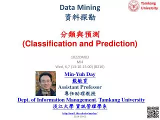
Tamkang University. 分類與預測 (Classification and Prediction). Data Mining 資料探勘. 1022DM03 MI4 Wed, 6,7 (13:10-15:00) (B216). Min-Yuh Day 戴敏育 Assistant Professor 專任助理教授 Dept. of Information Management , Tamkang University 淡江大學 資訊管理學系 http://mail. tku.edu.tw/myday/ 2014-03-05.

Data Mining 資料探勘
E N D
Presentation Transcript
Tamkang University 分類與預測 (Classification and Prediction) Data Mining資料探勘 1022DM03 MI4 Wed, 6,7 (13:10-15:00) (B216) Min-Yuh Day 戴敏育 Assistant Professor 專任助理教授 Dept. of Information Management, Tamkang University 淡江大學資訊管理學系 http://mail. tku.edu.tw/myday/ 2014-03-05
課程大綱 (Syllabus) 週次 (Week) 日期 (Date) 內容 (Subject/Topics) 1 103/02/19 資料探勘導論 (Introduction to Data Mining) 2 103/02/26 關連分析 (Association Analysis) 3 103/03/05 分類與預測 (Classification and Prediction) 4 103/03/12 分群分析 (Cluster Analysis) 5 103/03/19 個案分析與實作一 (SAS EM 分群分析):Case Study 1 (Cluster Analysis – K-Means using SAS EM) 6 103/03/26 個案分析與實作二 (SAS EM 關連分析): Case Study 2 (Association Analysis using SAS EM) 7 103/04/02 教學行政觀摩日 (Off-campus study) 8 103/04/09 個案分析與實作三 (SAS EM 決策樹、模型評估):Case Study 3 (Decision Tree, Model Evaluation using SAS EM)
課程大綱 (Syllabus) 週次 (Week) 日期 (Date) 內容 (Subject/Topics) 9 103/04/16 期中報告 (Midterm Project Presentation) 10 103/04/23 期中考試週 (Midterm Exam) 11 103/04/30 個案分析與實作四(SAS EM 迴歸分析、類神經網路):Case Study 4 (Regression Analysis, Artificial Neural Network using SAS EM) 12 103/05/07 文字探勘與網頁探勘 (Text and Web Mining) 13 103/05/14 海量資料分析 (Big Data Analytics) 14 103/05/21 期末報告 (Final Project Presentation) 15 103/05/28 畢業考試週 (Final Exam)
Outline Classification and Prediction Decision Tree Support Vector Machine (SVM) Evaluation (Accuracy of Classification Model) Source: Han & Kamber (2006)
Data Mining at the Intersection of Many Disciplines Source: Turban et al. (2011), Decision Support and Business Intelligence Systems
A Taxonomy for Data Mining Tasks Source: Turban et al. (2011), Decision Support and Business Intelligence Systems
Classification vs. Prediction • Classification • predicts categorical class labels (discrete or nominal) • classifies data (constructs a model) based on the training set and the values (class labels) in a classifying attribute and uses it in classifying new data • Prediction • models continuous-valued functions • i.e., predicts unknown or missing values • Typical applications • Credit approval • Target marketing • Medical diagnosis • Fraud detection Source: Han & Kamber (2006)
Data Mining Methods: Classification Most frequently used DM method Part of the machine-learning family Employ supervised learning Learn from past data, classify new data The output variable is categorical (nominal or ordinal) in nature Classification versus regression? Classification versus clustering? Source: Turban et al. (2011), Decision Support and Business Intelligence Systems
Classification Techniques Decision tree analysis Statistical analysis Neural networks Support vector machines Case-based reasoning Bayesian classifiers Genetic algorithms Rough sets Source: Turban et al. (2011), Decision Support and Business Intelligence Systems
Example of Classification • Loan Application Data • Which loan applicants are “safe” and which are “risky” for the bank? • “Safe” or “risky” for load application data • Marketing Data • Whether a customer with a given profile will buy a new computer? • “yes” or “no” for marketing data • Classification • Data analysis task • A model or Classifier is constructed to predict categorical labels • Labels: “safe” or “risky”; “yes” or “no”; “treatment A”, “treatment B”, “treatment C” Source: Han & Kamber (2006)
What Is Prediction? • (Numerical) prediction is similar to classification • construct a model • use model to predict continuous or ordered value for a given input • Prediction is different from classification • Classification refers to predict categorical class label • Prediction models continuous-valued functions • Major method for prediction: regression • model the relationship between one or more independent or predictor variables and a dependent or response variable • Regression analysis • Linear and multiple regression • Non-linear regression • Other regression methods: generalized linear model, Poisson regression, log-linear models, regression trees Source: Han & Kamber (2006)
Linear Regression Nonlinear Regression Other Regression Methods Prediction Methods Source: Han & Kamber (2006)
Classification and Prediction • Classification and prediction are two forms of data analysis that can be used to extract models describing important data classes or to predict future data trends. • Classification • Effective and scalable methods have been developed for decision trees induction, Naive Bayesian classification, Bayesian belief network, rule-based classifier, Backpropagation, Support Vector Machine (SVM), associative classification, nearest neighbor classifiers, and case-based reasoning, and other classification methods such as genetic algorithms, rough set and fuzzy set approaches. • Prediction • Linear, nonlinear, and generalized linear models of regression can be used for prediction. Many nonlinear problems can be converted to linear problems by performing transformations on the predictor variables. Regression trees and model trees are also used for prediction. Source: Han & Kamber (2006)
Classification—A Two-Step Process • Model construction: describing a set of predetermined classes • Each tuple/sample is assumed to belong to a predefined class, as determined by the class label attribute • The set of tuples used for model construction is training set • The model is represented as classification rules, decision trees, or mathematical formulae • Model usage: for classifying future or unknown objects • Estimate accuracy of the model • The known label of test sample is compared with the classified result from the model • Accuracy rate is the percentage of test set samples that are correctly classified by the model • Test set is independent of training set, otherwise over-fitting will occur • If the accuracy is acceptable, use the model to classify data tuples whose class labels are not known Source: Han & Kamber (2006)
Supervised vs. Unsupervised Learning • Supervised learning (classification) • Supervision: The training data (observations, measurements, etc.) are accompanied by labels indicating the class of the observations • New data is classified based on the training set • Unsupervised learning(clustering) • The class labels of training data is unknown • Given a set of measurements, observations, etc. with the aim of establishing the existence of classes or clusters in the data Source: Han & Kamber (2006)
Issues Regarding Classification and Prediction: Data Preparation • Data cleaning • Preprocess data in order to reduce noise and handle missing values • Relevance analysis (feature selection) • Remove the irrelevant or redundant attributes • Attribute subset selection • Feature Selection in machine learning • Data transformation • Generalize and/or normalize data • Example • Income: low, medium, high Source: Han & Kamber (2006)
Issues: Evaluating Classification and Prediction Methods • Accuracy • classifier accuracy: predicting class label • predictor accuracy: guessing value of predicted attributes • estimation techniques: cross-validation and bootstrapping • Speed • time to construct the model (training time) • time to use the model (classification/prediction time) • Robustness • handling noise and missing values • Scalability • ability to construct the classifier or predictor efficiently given large amounts of data • Interpretability • understanding and insight provided by the model Source: Han & Kamber (2006)
Data Classification Process 1: Learning (Training) Step (a) Learning: Training data are analyzed by classification algorithm y= f(X) Source: Han & Kamber (2006)
Data Classification Process 2 (b) Classification: Test data are used to estimate the accuracy of the classification rules. Source: Han & Kamber (2006)
Training Data Classifier (Model) Process (1): Model Construction Classification Algorithms IF rank = ‘professor’ OR years > 6 THEN tenured = ‘yes’ Source: Han & Kamber (2006)
Classifier Testing Data Unseen Data Process (2): Using the Model in Prediction (Jeff, Professor, 4) Tenured? Source: Han & Kamber (2006)
Decision Trees A general algorithm for decision tree building • Employs the divide and conquer method • Recursively divides a training set until each division consists of examples from one class • Create a root node and assign all of the training data to it • Select the best splitting attribute • Add a branch to the root node for each value of the split. Split the data into mutually exclusive subsets along the lines of the specific split • Repeat the steps 2 and 3 for each and every leaf node until the stopping criteria is reached Source: Turban et al. (2011), Decision Support and Business Intelligence Systems
Decision Trees • DT algorithms mainly differ on • Splitting criteria • Which variable to split first? • What values to use to split? • How many splits to form for each node? • Stopping criteria • When to stop building the tree • Pruning (generalization method) • Pre-pruning versus post-pruning • Most popular DT algorithms include • ID3, C4.5, C5; CART; CHAID; M5 Source: Turban et al. (2011), Decision Support and Business Intelligence Systems
Decision Trees • Alternative splitting criteria • Gini index determines the purity of a specific class as a result of a decision to branch along a particular attribute/value • Used in CART • Information gain uses entropy to measure the extent of uncertainty or randomness of a particular attribute/value split • Used in ID3, C4.5, C5 • Chi-square statistics (used in CHAID) Source: Turban et al. (2011), Decision Support and Business Intelligence Systems
Classification by Decision Tree InductionTraining Dataset This follows an example of Quinlan’s ID3 (Playing Tennis) Source: Han & Kamber (2006)
Classification by Decision Tree Induction age? senior >40 middle_aged31..40 youth<=30 student? credit rating? fair excellent no yes Output: A Decision Tree for “buys_computer” yes yes no yes no buys_computer=“yes” or buys_computer=“no” Source: Han & Kamber (2006)
Three possibilities for partitioning tuples based on the splitting Criterion Source: Han & Kamber (2006)
Algorithm for Decision Tree Induction • Basic algorithm (a greedy algorithm) • Tree is constructed in a top-down recursive divide-and-conquer manner • At start, all the training examples are at the root • Attributes are categorical (if continuous-valued, they are discretized in advance) • Examples are partitioned recursively based on selected attributes • Test attributes are selected on the basis of a heuristic or statistical measure (e.g., information gain) • Conditions for stopping partitioning • All samples for a given node belong to the same class • There are no remaining attributes for further partitioning – majority voting is employed for classifying the leaf • There are no samples left Source: Han & Kamber (2006)
Attribute Selection Measure • Notation: Let D, the data partition, be a training set of class-labeled tuples. Suppose the class label attribute has m distinct values defining m distinct classes, Ci (for i = 1, … , m). Let Ci,D be the set of tuples of class Ci in D. Let |D| and | Ci,D | denote the number of tuples in D and Ci,D , respectively. • Example: • Class: buys_computer= “yes” or “no” • Two distinct classes (m=2) • Class Ci (i=1,2): C1 = “yes”,C2 = “no” Source: Han & Kamber (2006)
Attribute Selection Measure: Information Gain (ID3/C4.5) • Select the attribute with the highest information gain • Let pi be the probability that an arbitrary tuple in D belongs to class Ci, estimated by |Ci, D|/|D| • Expected information (entropy) needed to classify a tuple in D: • Information needed (after using A to split D into v partitions) to classify D: • Information gained by branching on attribute A Source: Han & Kamber (2006)
Class-labeled training tuples from the AllElectronics customer database The attribute age has the highest information gain and therefore becomes the splitting attribute at the root node of the decision tree Source: Han & Kamber (2006)
Class P: buys_computer = “yes” Class N: buys_computer = “no” means “age <=30” has 5 out of 14 samples, with 2 yes’es and 3 no’s. Hence Similarly, Attribute Selection: Information Gain Source: Han & Kamber (2006)
Gain Ratio for Attribute Selection (C4.5) • Information gain measure is biased towards attributes with a large number of values • C4.5 (a successor of ID3) uses gain ratio to overcome the problem (normalization to information gain) • GainRatio(A) = Gain(A)/SplitInfo(A) • Ex. • gain_ratio(income) = 0.029/0.926 = 0.031 • The attribute with the maximum gain ratio is selected as the splitting attribute Source: Han & Kamber (2006)
Gini index (CART, IBM IntelligentMiner) • If a data set D contains examples from n classes, gini index, gini(D) is defined as where pj is the relative frequency of class j in D • If a data set D is split on A into two subsets D1 and D2, the gini index gini(D) is defined as • Reduction in Impurity: • The attribute provides the smallest ginisplit(D) (or the largest reduction in impurity) is chosen to split the node (need to enumerate all the possible splitting points for each attribute) Source: Han & Kamber (2006)
Gini index (CART, IBM IntelligentMiner) • Ex. D has 9 tuples in buys_computer = “yes” and 5 in “no” • Suppose the attribute income partitions D into 10 in D1: {low, medium} and 4 in D2 but gini{medium,high} is 0.30 and thus the best since it is the lowest • All attributes are assumed continuous-valued • May need other tools, e.g., clustering, to get the possible split values • Can be modified for categorical attributes Source: Han & Kamber (2006)
Comparing Attribute Selection Measures • The three measures, in general, return good results but • Information gain: • biased towards multivalued attributes • Gain ratio: • tends to prefer unbalanced splits in which one partition is much smaller than the others • Gini index: • biased to multivalued attributes • has difficulty when # of classes is large • tends to favor tests that result in equal-sized partitions and purity in both partitions Source: Han & Kamber (2006)
Classification in Large Databases • Classification—a classical problem extensively studied by statisticians and machine learning researchers • Scalability: Classifying data sets with millions of examples and hundreds of attributes with reasonable speed • Why decision tree induction in data mining? • relatively faster learning speed (than other classification methods) • convertible to simple and easy to understand classification rules • can use SQL queries for accessing databases • comparable classification accuracy with other methods Source: Han & Kamber (2006)
SVM—Support Vector Machines • A new classification method for both linear and nonlinear data • It uses a nonlinear mapping to transform the original training data into a higher dimension • With the new dimension, it searches for the linear optimal separating hyperplane (i.e., “decision boundary”) • With an appropriate nonlinear mapping to a sufficiently high dimension, data from two classes can always be separated by a hyperplane • SVM finds this hyperplane using support vectors (“essential” training tuples) and margins (defined by the support vectors) Source: Han & Kamber (2006)
SVM—History and Applications • Vapnik and colleagues (1992)—groundwork from Vapnik & Chervonenkis’ statistical learning theory in 1960s • Features: training can be slow but accuracy is high owing to their ability to model complex nonlinear decision boundaries (margin maximization) • Used both for classification and prediction • Applications: • handwritten digit recognition, object recognition, speaker identification, benchmarking time-series prediction tests, document classification Source: Han & Kamber (2006)
Small Margin Large Margin Support Vectors SVM—General Philosophy Source: Han & Kamber (2006)
Classification (SVM) The 2-D training data are linearly separable. There are an infinite number of (possible) separating hyperplanes or “decision boundaries.”Which one is best? Source: Han & Kamber (2006)
Classification (SVM) Which one is better? The one with the larger margin should have greater generalization accuracy. Source: Han & Kamber (2006)
SVM—When Data Is Linearly Separable m Let data D be (X1, y1), …, (X|D|, y|D|), where Xi is the set of training tuples associated with the class labels yi There are infinite lines (hyperplanes) separating the two classes but we want to find the best one (the one that minimizes classification error on unseen data) SVM searches for the hyperplane with the largest margin, i.e., maximum marginal hyperplane (MMH) Source: Han & Kamber (2006)
SVM—Linearly Separable • A separating hyperplane can be written as W ● X + b = 0 where W={w1, w2, …, wn} is a weight vector and b a scalar (bias) • For 2-D it can be written as w0 + w1 x1 + w2 x2 = 0 • The hyperplane defining the sides of the margin: H1: w0 + w1 x1 + w2 x2 ≥ 1 for yi = +1, and H2: w0 + w1 x1 + w2 x2 ≤ – 1 for yi = –1 • Any training tuples that fall on hyperplanes H1 or H2 (i.e., the sides defining the margin) are support vectors • This becomes a constrained (convex) quadratic optimization problem: Quadratic objective function and linear constraints Quadratic Programming (QP) Lagrangian multipliers Source: Han & Kamber (2006)
Why Is SVM Effective on High Dimensional Data? • The complexity of trained classifier is characterized by the # of support vectors rather than the dimensionality of the data • The support vectors are the essential or critical training examples —they lie closest to the decision boundary (MMH) • If all other training examples are removed and the training is repeated, the same separating hyperplane would be found • The number of support vectors found can be used to compute an (upper) bound on the expected error rate of the SVM classifier, which is independent of the data dimensionality • Thus, an SVM with a small number of support vectors can have good generalization, even when the dimensionality of the data is high Source: Han & Kamber (2006)
SVM—Linearly Inseparable • Transform the original input data into a higher dimensional space • Search for a linear separating hyperplane in the new space Source: Han & Kamber (2006)
Mapping Input Space to Feature Space Source: http://www.statsoft.com/textbook/support-vector-machines/
SVM—Kernel functions • Instead of computing the dot product on the transformed data tuples, it is mathematically equivalent to instead applying a kernel function K(Xi, Xj) to the original data, i.e., K(Xi, Xj) = Φ(Xi) Φ(Xj) • Typical Kernel Functions • SVM can also be used for classifying multiple (> 2) classes and for regression analysis (with additional user parameters) Source: Han & Kamber (2006)

