Advanced Linear Models, Contrasts, and F-Tests in Statistical Mapping

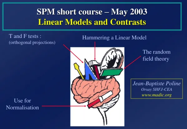
SPM short course – May 2003Linear Models and Contrasts T and F tests : (orthogonal projections) Hammering a Linear Model The random field theory Jean-Baptiste Poline Orsay SHFJ-CEA www.madic.org Use for Normalisation

Adjusted data Your question: a contrast Statistical Map Uncorrected p-values Design matrix images Spatial filter • General Linear Model • Linear fit • statistical image realignment & coregistration Random Field Theory smoothing normalisation Anatomical Reference Corrected p-values

Make sure we know all about the estimation (fitting) part .... Plan • Make sure we understand the testing procedures : t- and F-tests • A bad model ... And a better one • Correlation in our model : do we mind ? • A (nearly) real example

One voxel = One test (t, F, ...) amplitude • General Linear Model • fitting • statistical image time Statistical image (SPM) Temporal series fMRI voxel time course

90 100 110 -10 0 10 90 100 110 -2 0 2 m a m = 100 a = 1 Fit the GLM Mean value voxel time series box-car reference function Regression example… + + =

90 100 110 90 100 110 -2 0 2 -2 0 2 m a m = 100 a = 5 Mean value error voxel time series box-car reference function Regression example… + + =

…revisited : matrix form = a m + + error Ys m 1 a f(ts) es = + + ´ ´

Box car regression: design matrix… data vector (voxel time series) parameters error vector design matrix a = ´ + m ´ Y = X b + e

Add more reference functions ... Discrete cosine transform basis functions

…design matrix = the betas (here : 1 to 9) parameters error vector design matrix data vector a m b3 b4 b5 b6 b7 b8 b9 = + ´ = + Y X b e

S = s2 the squared values of the residuals number of time points minus the number of estimated betas Fitting the model = finding some estimate of the betas= minimising the sum of square of the residuals S2 raw fMRI time series adjusted for low Hz effects fitted box-car fitted “high-pass filter” residuals

Summary ... • We put in our model regressors (or covariates) that represent how we think the signal is varying (of interest and of no interest alike) • Coefficients (=parameters) are estimated using the Ordinary Least Squares (OLS) or Maximum Likelihood (ML) estimator. • These estimated parameters (the “betas”) depend on the scaling of the regressors. • The residuals, their sum of squares and the resulting tests (t,F), do not depend on the scaling of the regressors.

Plan • Make sure we all know about the estimation (fitting) part .... • Make sure we understand t and F tests • A bad model ... And a better one • Correlation in our model : do we mind ? • A (nearly) real example

c’ = 1 0 0 0 0 0 0 0 contrast ofestimatedparameters c’b T = T = varianceestimate s2c’(X’X)+c SPM{t} T test - one dimensional contrasts - SPM{t} A contrast= a linear combination of parameters: c´´b box-car amplitude > 0 ? = b1 > 0 ? => b1b2b3b4b5.... Compute 1xb1+ 0xb2+ 0xb3+ 0xb4+ 0xb5+ . . . and divide by estimated standard deviation

^ b Estimation [Y, X] [b, s] Y = X b + ee ~ s2 N(0,I)(Y : at one position) b = (X’X)+ X’Y (b: estimate of b) -> beta??? images e = Y - Xb(e: estimate of e) s2 = (e’e/(n - p)) (s: estimate of s, n: time points, p: parameters) -> 1 image ResMS Test [b, s2, c] [c’b, t] Var(c’b) = s2c’(X’X)+c (compute for each contrast c) t = c’b / sqrt(s2c’(X’X)+c) (c’b -> images spm_con??? compute the t images -> images spm_t??? ) under the null hypothesis H0 : t ~ Student-t( df ) df = n-p contrast ofestimatedparameters How is this computed ? (t-test) varianceestimate

additionalvarianceaccounted forby tested effects X0 F = errorvarianceestimate S02 F ~ (S02 - S2 ) /S2 Or this one? F-test (SPM{F}) : a reduced model or ... Tests multiple linear hypotheses : Does X1 model anything ? H0: True (reduced) model is X0 X0 X1 S2 This (full) model ?

H0: True model is X0 0 0 1 0 0 0 0 0 0 0 0 1 0 0 0 0 0 0 0 0 1 0 0 0 0 0 0 0 0 1 0 0 0 0 0 0 0 0 1 0 0 0 0 0 0 0 0 1 X0 X0 X1(b3-9) c’ = This model ? Or this one ? F-test (SPM{F}) : a reduced model or ...multi-dimensional contrasts ? tests multiple linear hypotheses. Ex : does DCT set model anything? test H0 : c´´ b = 0 ? H0: b3-9 = (0 0 0 0 ...) SPM{F}

Estimation [Y, X] [b, s] Y=X b + ee ~ N(0, s2 I) Y=X0b0+ e0e0 ~ N(0, s02 I) X0 : X Reduced Estimation [Y, X0] [b0, s0] b0 = (X0’X0)+ X0’Y e0 = Y - X0 b0(eà: estimate of eà) s20 = (e0’e0/(n - p0)) (sà: estimate of sà, n: time, pà: parameters) Test [b, s, c] [ess, F] F = (e0’e0 - e’e)/(p - p0) / s2 -> image (e0’e0 - e’e)/(p - p0) : spm_ess??? -> image of F : spm_F??? under the null hypothesis : F ~ F(df1,df2) p - p0 n-p additionalvariance accounted forby tested effects How is this computed ? (F-test) Error varianceestimate

True signal and observed signal (---) Model (green, pic at 6sec) TRUE signal (blue, pic at 3sec) Fitting (b1 = 0.2, mean = 0.11) Residual(still contains some signal) => Test for the green regressor not significant A bad model ...

A bad model ... b1= 0.22 b2= 0.11 Residual Variance = 0.3 P(Y|b1= 0) => p-value = 0.1 (t-test) P(Y|b1= 0) => p-value = 0.2 (F-test) = + Y X b e

True signal + observed signal Model (green and red) and true signal (blue ---) Red regressor : temporal derivative of the green regressor Global fit (blue) and partial fit (green & red) Adjusted and fitted signal Residual(a smaller variance) => t-test of the green regressor significant => F-test very significant => t-test of the red regressor very significant A « better » model ...

A better model ... b1= 0.22 b2= 2.15 b3= 0.11 Residual Var = 0.2 P(Y|b1= 0) p-value = 0.07 (t-test) P(Y|b1= 0, b2= 0) p-value = 0.000001 (F-test) = + Y X b e

Flexible models :Fourier Transform Basis

Flexible models : Gamma Basis

Summary ... (2) • The residuals should be looked at ...(non random structure ?) • We rather test flexible models if there is little a priori information, and precise ones with a lot a priori information • In general, use the F-tests to look for an overall effect, then look at the betas or the adjusted data to characterise the response shape • Interpreting the test on a single parameter (one regressor) can be difficult: cf the delay or magnitude situation

Plan • Make sure we all know about the estimation (fitting) part .... • Make sure we understand t and F tests • A bad model ... And a better one • Correlation in our model : do we mind ? • A (nearly) real example ?

Model (green and red) Fit (blue : global fit) Residual Correlation between regressors True signal

Correlation between regressors b1= 0.79 b2= 0.85 b3 = 0.06 Residual var. = 0.3 P(Y|b1= 0) p-value = 0.08 (t-test) P(Y|b2= 0) p-value = 0.07 (t-test) P(Y|b1= 0, b2= 0) p-value = 0.002 (F-test) = + Y X b e

Model (green and red) red regressor has been orthogonalised with respect to the green one  remove everything that correlates with the green regressor Fit Residual Correlation between regressors - 2 true signal

Correlation between regressors -2 0.79 0.85 0.06 b1= 1.47 b2= 0.85 b3 = 0.06 Residual var. = 0.3 P(Y|b1= 0) p-value = 0.0003 (t-test) P(Y|b2= 0) p-value = 0.07 (t-test) P(Y|b1= 0, b2= 0) p-value = 0.002 (F-test) = + Y X b e See « explore design »

1 2 1 2 1 1 2 2 1 1 2 2 Design orthogonality : « explore design » Black = completely correlated White = completely orthogonal Corr(1,1) Corr(1,2) Beware: when there are more than 2 regressors (C1,C2,C3,...), you may think that there is little correlation (light grey) between them, but C1 + C2 + C3 may be correlated with C4 + C5

Xb Y C2 C1 e Xb Space of X C2 C1 C2 Xb C2^ LC1^ C1 LC2 LC2 : test of C2 in the implicit ^ model LC1^ : test of C1 in the explicit ^ model ^ Implicit or explicit (^)decorrelation (or orthogonalisation) This GENERALISES when testing several regressors (F tests) See Andrade et al., NeuroImage, 1999

^ b ? 1 0 1 0 1 1 1 0 1 0 1 1 X = Y = Xb + e Mean Cond 1 Cond 2 “completely” correlated ... Mean = C1+C2 C2 C1 Parameters are not unique in general ! Some contrasts have no meaning: NON ESTIMABLE Example here : c’ = [1 0 0] is not estimable ( = no specific information in the first regressor); c’ = [1 -1 0] is estimable;

Summary ... (3) • We implicitly test for an additional effect only, so we may miss the signal if there is some correlation in the model • Orthogonalisation is not generally needed - parameters and test on the changed regressor don’t change • It is always simpler (if possible!) to have orthogonal regressors • In case of correlation, use F-tests to see the overall significance. There is generally no way to decide to which regressor the « common » part should be attributed to • In case of correlation and if you need to orthogonolise a part of the design matrix, there is no need to re-fit a new model: change the contrast

C1 V A C1 C2 C3 V C2 C3 C1 C2 A C3 A real example (almost !) Experimental Design Design Matrix Factorial design with 2 factors : modality and category 2 levels for modality (eg Visual/Auditory) 3 levels for category (eg 3 categories of words)

Asking ourselves some questions ... V A C1 C2 C3 2 ways : 1- write a contrast c and test c’b = 0 2- select columns of X for the model under the null hypothesis. Test C1 > C2 : c = [ 0 0 1 -1 0 0 ] Test V > A : c = [ 1 -1 0 0 0 0 ] Test the modality factor : c = ? Test the category factor : c = ? Test the interaction MxC ? • Design Matrix not orthogonal • Many contrasts are non estimable • Interactions MxC are not modelled

Modelling the interactions

Asking ourselves some questions ... C1 C1 C2 C2 C3 C3 Test C1 > C2 : c = [ 1 1 -1 -1 0 0 0] Test V > A : c = [ 1 -1 1 -1 1 -1 0] Test the differences between categories : [ 1 1 -1 -1 0 0 0] c = [ 0 0 1 1 -1 -1 0] V A V A V A Test everything in the category factor , leave out modality : [ 1 1 0 0 0 0 0] c = [ 0 0 1 1 0 0 0] [ 0 0 0 0 1 1 0] Test the interaction MxC : [ 1 -1 -1 1 0 0 0] c = [ 0 0 1 -1 -1 1 0] [ 1 -1 0 0 -1 1 0] • Design Matrix orthogonal • All contrasts are estimable • Interactions MxC modelled • If no interaction ... ? Model too “big”

Asking ourselves some questions ... With a more flexible model C1 C1 C2 C2 C3 C3 V A V A V A Test C1 > C2 ? Test C1 different from C2 ? from c = [ 1 1 -1 -1 0 0 0] to c = [ 1 0 1 0 -1 0 -1 0 0 0 0 0 0] [ 0 1 0 1 0 -1 0 -1 0 0 0 0 0] becomes an F test! Test V > A ? c = [ 1 0 -1 0 1 0 -1 0 1 0 -1 0 0] is possible, but is OK only if the regressors coding for the delay are all equal

Conclusion • Check your models • Toolbox of T. Nichols • Multivariate Methods toolbox (F. Kherif, JB Poline et al) • Check the form of the HRF : non parametric estimation www.fil.ion.ucl.ac.uk; www.madic.org; others …

Advanced Linear Models, Contrasts, and F-Tests in Statistical Mapping