Download

1 / 34
340 likes | 379 Vues
This lecture explores AVL trees, a type of self-balancing binary search tree. Learn about balanced BSTs, balance factors, height-balanced trees, and the operations involved in AVL trees.

E N D
Lecture 23 AVL tree Chapter 10 of textbook 1. Binary Search Tree (BST) • Threaded Tree • AVL Tree • Red Black Tree • Splay Tree
Balanced BST Balanced BST, i.e. height of left and right subtrees are equal or not much differences at any nodeExample: a full binary tree of n nodes is balanced treeThe search in can be done in log(n) time, O(log n). Depth of recursion is O(log n) Time complexity O(log n) Space complexity O(log n) A BST is not balanced in general !
Balance factor • The balance factor of a node is calculated by subtracting the height of its right sub-tree from the height of its left sub-tree. Balance factor = Height (left sub-tree) – Height (right sub-tree)
Balance factor • If the balance factor of a node is 1, then it means that the left sub-tree of the tree is one level higher than that of the right sub-tree. Such a tree is called Left-heavy tree. • If the balance factor of a node is 0, then it means that the height of the left sub-tree is equal to the height of its right sub-tree. • If the balance factor of a node is -1, then it means that the left sub-tree of the tree is one level lower than that of the right sub-tree. Such a tree is called Right-heavy tree. • A node is unbalanced if its balance factor is not -1, 0, or 1.
Examples of Balance Factor -1 45 0 -1 36 63 0 1 0 0 27 72 39 54 0 70 0 45 0 0 36 63 0 1 0 0 45 27 0 39 54 72 1 36 63 0 0 27 1 39 54 72 0 0 18 0 Balanced AVL tree Left heavy AVL tree Right heavy AVL tree
Height Balanced Tree • A binary search tree in which every node has a balance factor of -1, 0 or 1 is said to be height balanced. In another word: at any node, the difference of heights of two sub-trees is at most 1 • Property: height of balanced tree of n nodes is O(log n).
Height Balanced Tree Property: height of balanced tree of n nodes is O(log n). Proof: 𝑁(ℎ) denote the minimum number of AVL tree of height h, then 𝑁(ℎ) <= n 𝑁(ℎ)=1+𝑁(ℎ−1)+𝑁(ℎ−2) We may assume that 𝑁(ℎ−1)>𝑁(ℎ−2), 𝑁(ℎ)>1+𝑁(ℎ−2)+𝑁(ℎ−2)=1+2⋅𝑁(ℎ−2)>2⋅𝑁(ℎ−2) 𝑁(ℎ)>2⋅𝑁(ℎ−2) 𝑁(ℎ)>2⋅𝑁(ℎ−2)>2⋅2⋅𝑁(ℎ−4)>2⋅2⋅2⋅𝑁(ℎ−6)>⋯>2ℎ/2 log𝑁(ℎ) > log 2ℎ/2 ℎ < 2 log 𝑁(ℎ) <= 2 log n Thus, these worst-case AVL trees have height ℎ = O(log𝑛).
Height Balanced Tree -1 45 0 -1 36 63 0 1 0 0 27 72 39 54 0 70 0 45 0 0 36 63 0 1 0 0 45 27 0 39 54 72 1 36 63 0 2 45 -1 0 27 1 36 63 0 39 54 72 0 0 27 -1 0 18 0 -1 42 YES YES NO YES 39
3. AVL Trees • AVL tree is a self-balancing binary search tree in which the heights of the two sub-trees of a node may differ by at most one. • AVL tree is a height-balanced tree • Self-balancing : re-balance after BST inserting or deleting • AVL is named by its inventor Adelson-Velskii and Landis • provided the height balance property and insertion and deletion operations that maintain the property in time complexity of O(log n)
Features of AVL Trees • The key advantage of using an AVL tree is that it takes O(log n) time to perform search, insertion and deletion operations in average case as well as worst case (because the height of the tree is limited to O(log n). • The structure of an AVL tree is same as that of a binary search tree but with a little difference. In its structure, it stores an additional variable called the Balance Factor.
Searching for a Node in an AVL Tree • Searching in an AVL tree is performed exactly the same way as it is performed in a binary search tree. • Because of the height-balancing of the tree, the search operation takes O(log n) time to complete. • Since the operation does not modify the structure of the tree, no special provisions need to be taken.
Inserting a Node in an AVL Tree • Algorithm: Step 1. insert new node as BST Step 2: if not AVL tree, do re-balancing to derive an AVL tree • A new node is inserted as the leaf node, so it will always have balance factor equal to zero. • The nodes whose balance factors will change are those which lie on the path between the root of the tree and the newly inserted node.
Inserting a Node in an AVL Tree • The possible changes which may take place in any node on the path are as follows: • Initially the node was either left or right heavy and after insertion has become balanced. • Initially the node was balanced and after insertion has become either left or right heavy. • Initially the node was heavy (either left or right) and the new node has been inserted in the heavy sub-tree thereby creating an unbalanced sub-tree. Such a node is said to be a critical node. • The critical node is the unbalanced node of lowest level
Example of critical node 2 45 2 36 63 0 2 0 27 39 54 72 0 1 18 0 0 9 1 45 1 36 63 0 1 0 27 39 54 72 0 0 18 0 Example: Consider the AVL tree given below and insert 9 into it. Critical node
Example of AVL tree insert Insert 50, 25, 10, 5, 7, 3, 30, 20, 8, 15 into AVL tree
Example of AVL tree insert Insert 50, 25, 10, 5, 7, 3, 30, 20, 8, 15 into AVL tree
Cases of critical nodes • Height of sub-tree where a new node is inserted can increase at most 1. • The balance factor can crease by 1 or decrease by 1, so the balance factor of critical node is either 2 or -2. Let x denote the critical node. There are four possible cases: Case 1: balance-factor(x) = 2, balance-factor(x->left) >=0, Case 2: balance-factor(x) = 2, balance-factor(x->left) < 0, Case 3: balance-factor(x) = -2, balance-factor(x->right) < =0, Case 4: balance-factor(x) = -2, balance-factor(x->right) >0 Each case will different rotation operation for re-balancing
Case 1: right-rotation to re-balance Case 1: balance-factor(x) = 2, balance-factor(x->left) >= 0right_rotation(x) it return y as new top node x h+2 y h+1 2 0 y h+1 T3 h-1 T1 h x h right-rotation 1 0 T1h T2 h-1 T3 h-1 T2 h-1
L-R-Rotation for Re-balancing Case 2 balance-factor(x) = 2, balance-factor(x->left) < 0 x->left = left_rotate(x->left); right_rotation(x); x x y z z T4 T4 2 y y x T3 z T1 -1 left-rotation right-rotation T1 T1 T2 T2 T3 T2 T3 T4
left-rotation to re-balance Case 3: balance-factor(x) = -2, balance-factor(x->right) <= 0left_rotation(x); y h+1 x h+2 -2 0 left-rotation x h T3 h T1 h-1 y h+1 0 -1 T1h-1 T2 h-1 T3 h T2 h-1
R-L-Rotation re-balancing x x Case 4. balance-factor(x) = -2, balance-factor(x->right) > 0 x->right = right_rotate(x->right); left_rotation(x); y T1 T1 z z -2 right-rotation left-rotation 1 z T4 y x y T2 T2 T3 T3 T4 T1 T2 T3 T4
Case 2: R-Rotations to Balance AVL Tree 2 45 2 36 63 0 2 0 27 39 54 72 0 1 18 0 0 9 1 45 0 27 63 0 1 0 18 36 54 72 0 0 0 9 0 39 1 45 1 36 63 0 1 0 27 39 54 72 0 0 18 0 Example: Consider the AVL tree given below and insert 9 into it. LL case Critical node The tree is balanced using R-rotation
Case 2: L-R-Rotation -2 -1 -1 45 45 45 36 36 36 63 63 63 -1 -2 -1 27 27 27 2 1 1 39 39 39 54 54 54 72 72 70 69 69 69 Example: Consider the AVL tree given below and insert 70 into it. 72 The tree is balanced using L-R- rotation -1 70
Case 3. L-Rotation to Balance -1 45 0 36 72 0 -2 45 0 -1 0 27 39 63 89 36 63 -2 -1 0 0 27 -2 0 54 91 0 39 54 72 0 -1 89 -1 45 0 0 91 36 63 -1 0 0 27 -1 39 54 72 0 0 89 Example: Consider the AVL tree given below and insert 91 into it. RR-case The tree is balanced using L-rotation
Case 4. R-L-Rotation to Balance 2 1 2 45 45 45 -2 -2 -1 36 36 36 63 63 63 0 0 0 0 0 0 0 0 0 27 27 27 39 39 54 54 54 72 72 72 0 0 0 -1 -2 42 42 42 0 -1 Example: Consider the AVL tree given below and insert 40 into it. 40 39 Critical node The tree is balanced using R-L rotation 40
Deleting a Node from an AVL Tree • Deleting algorithm Step 1. delete node as BST Step 2. if not height balanced, rebalance by rotation If the resulting BST of step 1 is not height-balanced, find the critical node. There are four possible cases similar to the inserting. Then do corresponding rotation by the case
Rotate to rebalance Case 1: balance-factor(x) = 2, balance-factor(x->left) >=0, right_rotation(x);Case 2: balance-factor(x) = 2, balance-factor(x->left) < 0, x->left = left_rotate(x->left); right_rotation(x);Case 3: balance-factor(x) = -2, balance-factor(x->right) <=0, left_rotation(x); Case 4: balance-factor(x) = -2, balance-factor(x->right) >0x->right = right_rotate(x->right); left_rotation(x);
Deleting a Node from an AVL Tree 1 45 0 36 63 -1 1 27 -1 72 39 0 0 18 40 0 2 45 -1 36 1 36 63 0 27 45 1 1 0 27 -1 18 0 39 63 -1 0 0 18 40 0 40 Example: Consider the AVL tree given below and delete 72 from it. Case 1. R-rotation 0 39
Deleting a Node from an AVL Tree 1 45 -1 36 63 -1 0 0 0 27 39 72 0 0 41 37 1 2 39 45 1 36 45 1 36 63 0 0 1 0 0 0 27 39 27 37 41 63 0 0 0 37 41 • Consider the AVL tree given below and delete 72 from it. • Case 2. L-R-rotation -1
AVL implementation node design struct Node { int key; int height; // or using balance factor int data; // application data associated with key struct Node *left, *right; };
AVL right-rotate node *right_rotate(node *y) { node *x = y->left; node *T2 = x->right; // perform rotation x->right = y; y->left = T2; // Update heights y->height = max(height(y->left), height(y->right))+1; x->height = max(height(x->left), height(x->right))+1; return x; }http://www.geeksforgeeks.org/avl-tree-set-2-deletion/ y x / \ Right Rotation / \ x T3 – – – – – – – > T1 y / \ < - - - - - - - / \ T1 T2 Left Rotation T2 T3
AVL left-rotate node *left_rotate(node *x) { node *y = x->right; node *T2 = y->left; // perform rotation y->left = x; x->right = T2; // Update heights x->height = max(height(x->left), height(x->right))+1; y->height = max(height(y->left), height(y->right))+1; return y; } y x / \ Right Rotation / \ x T3 – – – – – – – > T1 y / \ < - - - - - - - / \ T1 T2 Left Rotation T2 T3
AVL insert node* insert(node* root, int key) { if (root == NULL) return(new_node(key)); if (key < root->key) root->left = insert(root->left, key); else if (key > root->key) root->right = insert(root->right, key); else return root; root->height = 1 + max(height(root->left), height(root->right)); int balance = balance_factor(root); // do rotation by cases
AVL implementation insert if (balance > 1 && balance_factor(root->left) >=0 ) return right_rotate(root); if (balance < -1 && balance_factor(root->left) <=0 ) return left_rotate(root); if (balance > 1 && balance_factor(root->left) < 0) { root->left = left_rotate(root->left); return right_rotate(root); } if (balance < -1 && balance_factor(root->left) > 0) { root->right = right_rotate(root->right); return left_rotate(root); } return root; }