MAP Estimation in Gaussian Models: Understanding Prior Distribution
Learn about the Maximum A Posteriori (MAP) estimation in Gaussian models, focusing on prior distribution, likelihood function, and EM algorithm for parameter estimation in Hidden Markov Models (HMM). Understand the key issues and intricacies of MAP estimation in Gaussian settings.

MAP Estimation in Gaussian Models: Understanding Prior Distribution
E N D
Presentation Transcript
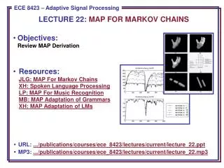
LECTURE 22: MAP FOR MARKOV CHAINS • Objectives:Review MAP Derivation • Resources:JLG: MAP For Markov ChainsXH: Spoken Language ProcessingLP: MAP For Music RecognitionMB: MAP Adaptation of GrammarsXH: MAP Adaptation of LMs • URL: .../publications/courses/ece_8423/lectures/current/lecture_22.ppt • MP3: .../publications/courses/ece_8423/lectures/current/lecture_22.mp3
Introduction • Consider the problem of estimating given a sequence of observations, o. The maximum a posteriori (MAP) estimate of is given by: • Three key issues need to be addressed: the choice of the prior distribution family, the specification of the parameters for the prior densities, and the evaluation of the MAP. • These problems are closely related since an appropriate choice of the prior distribution can greatly simplify the MAP estimation process. • For both finite mixture densities and hidden Markov models, EM must be used because the distribution lacks a sufficient statistic due to the underlying hidden process (i.e., the state mixture component and the state sequence of a Markov chain for an HMM). • For HMM parameter estimation, EM is known as the Baum-Welch (BW) algorithm and alternates between maximizing the likelihood function of the observed data and reestimating the parameters using expectations. • We will assume the data is generated from a multivariate Gaussian distribution, and the T observations are i.i.d. and independent. • We will ignore the use of mixture densities (see Gauvain, 1994 for the details).
The Likelihood Function • The likelihood of the data (with respect to the kth state) can be written as: • The matrix r is referred to as the precision matrix and is defined as the inverse of the covariance matrix. The constant terms in the Gaussian are ignored because they don’t affect the optimization. • The prior distribution for the Gaussian mean and covariance is approximated with a normal-Wishart distribution: • A Wishart distribution is a multidimensional generalization of the Chi-squared distribution. A Chi-squared distribution results from taking the sum of the squares of Gaussian random variables. • The vector and matrix, , are the prior density parameters for . • : number of degrees of freedom; : proportional to the prior prob.
MAP Estimates for a Gaussian • The EM algorithm can be applied to find the ML estimates. The auxiliary function, , that is maximized is the combination of: • The auxiliary function, , is given by: • Continue from the Gauvain paper.