Download
1 / 45
450 likes | 500 Vues
Learn about PCA, its history, geometric rationale, computation process, dissimilarity measures, and generalization to p-dimensional space for effective data summarization and representation.

E N D
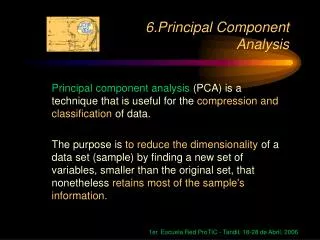
Data Reduction p k X A n n • summarization of data with many (p) variables by a smaller set of (k) derived (synthetic, composite) variables.
Data Reduction • “Residual” variation is information in A that is not retained in X • balancing act between • clarity of representation, ease of understanding • oversimplification: loss of important or relevant information.
Principal Component Analysis(PCA) • probably the most widely-used and well-known of the “standard” multivariate methods • invented by Pearson (1901) and Hotelling (1933) • first applied in ecology by Goodall (1954) under the name “factor analysis” (“principal factor analysis” is a synonym of PCA).
Principal Component Analysis(PCA) • takes a data matrix of n objects by p variables, which may be correlated, and summarizes it by uncorrelated axes (principal components or principal axes) that are linear combinations of the original p variables • the first k components display as much as possible of the variation among objects.
Geometric Rationale of PCA • objects are represented as a cloud of n points in a multidimensional space with an axis for each of the p variables • the centroidof the points is defined by the mean of each variable • the variance of each variable is the average squared deviation of its n values around the mean of that variable.
Geometric Rationale of PCA Covariance ofvariables i and j Mean ofvariable j Value of variable i in object m Value of variable j in object m Mean ofvariable i Sum over all n objects • degree to which the variables are linearly correlated is represented by their covariances.
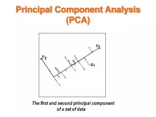
Geometric Rationale of PCA • objective of PCA is to rigidly rotate the axes of this p-dimensional space to new positions (principal axes) that have the following properties: • ordered such that principal axis 1 has the highest variance, axis 2 has the next highest variance, .... , and axis p has the lowest variance • covariance among each pair of the principal axes is zero (the principal axes are uncorrelated).
2D Example of PCA • variables X1and X2 have positive covariance & each has a similar variance.
Configuration is Centered • each variable is adjusted to a mean of zero (by subtracting the mean from each value).
Principal Components are Computed • PC 1 has the highest possible variance (9.88) • PC 2 has a variance of 3.03 • PC 1 and PC 2 have zero covariance.
The Dissimilarity Measure Used in PCA is Euclidean Distance • PCA uses Euclidean Distance calculated from the p variables as the measure of dissimilarity among the n objects • PCA derives the best possible k dimensional (k < p) representation of the Euclidean distances among objects.
Generalization to p-dimensions • In practice nobody uses PCA with only 2 variables • The algebra for finding principal axes readily generalizes to p variables • PC 1 is the direction of maximum variance in the p-dimensional cloud of points • PC 2 is in the direction of the next highest variance, subject to the constraint that it has zero covariance with PC 1.
Generalization to p-dimensions • PC 3 is in the direction of the next highest variance, subject to the constraint that it has zero covariance with both PC 1 and PC 2 • and so on... up to PC p
PC 1 PC 2 • each principal axis is a linear combination of the original two variables • PCj = ai1Y1 + ai2Y2 + … ainYn • aij’s are the coefficients for factor i, multiplied by the measured value for variable j
PC 1 PC 2 • PC axes are a rigid rotation of the original variables • PC 1 is simultaneously the direction of maximum variance and a least-squares “line of best fit” (squared distances of points away from PC 1 are minimized).
Generalization to p-dimensions • if we take the first k principal components, they define the k-dimensional “hyperplane of best fit” to the point cloud • of the total variance of all p variables: • PCs 1 to k represent the maximum possible proportion of that variance that can be displayed in k dimensions • i.e. the squared Euclidean distances among points calculated from their coordinates on PCs 1 to k are the best possible representation of their squared Euclidean distances in the full p dimensions.
Covariance vs Correlation Mean variable i Standard deviationof variable i • using covariances among variables only makes sense if they are measured in the same units • even then, variables with high variances will dominate the principal components • these problems are generally avoided by standardizing each variable to unit variance and zero mean.
Covariance vs Correlation Covariance of variables i and j Correlation betweenvariables i and j Varianceof variable j Varianceof variable i • covariances between the standardized variables are correlations • after standardization, each variable has a variance of 1.000 • correlations can be also calculated from the variances and covariances:
The Algebra of PCA • first step is to calculate the cross-products matrix of variances and covariances (or correlations) among every pair of the p variables • square, symmetric matrix • diagonals are the variances, off-diagonals are the covariances. Correlation Matrix Variance-covariance Matrix
The Algebra of PCA • in matrix notation, this is computed as • where X is the n x p data matrix, with each variable centered (also standardized by SD if using correlations). Correlation Matrix Variance-covariance Matrix
Manipulating Matrices • transposing: could change the columns to rows or the rows to columns • multiplying matrices • must have the same number of columns in the premultiplicand matrix as the number of rows in the postmultiplicand matrix X’ = 10 7 0 1 4 2 X = 10 0 4 7 1 2
The Algebra of PCA • sum of the diagonals of the variance-covariance matrix is called the trace • it represents the total variance in the data • it is the mean squared Euclidean distance between each object and the centroid in p-dimensional space. Trace = 2.0000 Trace = 12.9091
The Algebra of PCA • finding the principal axes involves eigenanalysis of the cross-products matrix (S) • the eigenvalues (latent roots) of S are solutions () to the characteristic equation
The Algebra of PCA • the eigenvalues, 1, 2, ... p are the variances of the coordinates on each principal component axis • the sum of all p eigenvalues equals the trace of S (the sum of the variances of the original variables). 1 = 9.8783 2 = 3.0308Note: 1+2 =12.9091 Trace = 12.9091
The Algebra of PCA • each eigenvector consists of p values which represent the “contribution” of each variable to the principal component axis • eigenvectors are uncorrelated (orthogonal) • their cross-products are zero. Eigenvectors 0.7291*(-0.6844) + 0.6844*0.7291 = 0
The Algebra of PCA • coordinates of each object i on the kthprincipal axis, known as the scores on PC k, are computed as • where Z is the n x k matrix of PC scores, X is the n x p centered data matrix and U is the p x k matrix of eigenvectors.
The Algebra of PCA • variance of the scores on each PC axis is equal to the corresponding eigenvalue for that axis • the eigenvalue represents the variance displayed (“explained” or “extracted”) by the kthaxis • the sum of the first k eigenvalues is the variance explained by the k-dimensional ordination.
1 = 9.8783 2 = 3.0308 Trace = 12.9091PC 1 displays (“explains”) 9.8783/12.9091 = 76.5% of the total variance
The Algebra of PCA • The cross-products matrix computed among the p principal axes has a simple form: • all off-diagonal values are zero (the principal axes are uncorrelated) • the diagonal values are the eigenvalues. Variance-covariance Matrixof the PC axes
A more challenging example • data from research on habitat definition in the endangered Baw Baw frog • 16 environmental and structural variables measured at each of 124 sites • correlation matrix used because variables have different units Philoria frosti
Interpreting Eigenvectors • correlations between variables and the principal axes are known as loadings • each element of the eigenvectors represents the contribution of a given variable to a component
How many axes are needed? • does the (k+1)thprincipal axis represent more variance than would be expected by chance? • several tests and rules have been proposed • a common “rule of thumb” when PCA is based on correlations is that axes with eigenvalues > 1 are worth interpreting
What are the assumptions of PCA? • assumes relationships among variables are LINEAR • cloud of points in p-dimensional space has linear dimensions that can be effectively summarized by the principal axes • if the structure in the data is NONLINEAR (the cloud of points twists and curves its way through p-dimensional space), the principal axes will not be an efficient and informative summary of the data.
When should PCA be used? • In community ecology, PCA is useful for summarizing variables whose relationships are approximately linear or at least monotonic • e.g. A PCA of many soil properties might be used to extract a few components that summarize main dimensions of soil variation • PCA is generally NOT useful for ordinating community data • Why? Because relationships among species are highly nonlinear.
The “Horseshoe” or Arch Effect • community trends along environmenal gradients appear as “horseshoes” in PCA ordinations • none of the PC axes effectively summarizes the trend in species composition along the gradient • SUs at opposite extremes of the gradient appear relatively close together.
The “Horseshoe”Effect • curvature of the gradient and the degree of infolding of the extremes increase with beta diversity • PCA ordinations are not useful summaries of community data except when beta diversity is very low • using correlation generally does better than covariance • this is because standardization by species improves the correlation between Euclidean distance and environmental distance.
What if there’s more than one underlying ecological gradient?
The “Horseshoe” Effect • when two or more underlying gradients with high beta diversity a “horseshoe” is usually not detectable • the SUs fall on a curved hypersurface that twists and turns through the p-dimensional species space • interpretation problems are more severe • PCA should NOT be used with community data (except maybe when beta diversity is very low).
Impact on Ordination History • by 1970 PCA was the ordination method of choice for community data • simulation studies by Swan (1970) & Austin & Noy-Meir (1971) demonstrated the horseshoe effect and showed that the linear assumption of PCA was not compatible with the nonlinear structure of community data • stimulated the quest for more appropriate ordination methods.