Principal Component Analysis (PCA)
Learn how PCA simplifies complex data, discovers trends, and reduces dimensions to focus on key information in data analysis.

Principal Component Analysis (PCA)
E N D
Presentation Transcript
Principal Component Analysis (PCA) BCH394P/364C Systems Biology / Bioinformatics Edward Marcotte, Univ of Texas at Austin
What is Principal Component Analysis? What does it do? So, first let’s build some intuition. “You do not really understand something unless you can explain it to your grandmother”, Albert Einstein wikipedia With thanks for many of these explanations to http://stats.stackexchange.com/questions/2691/making-sense-of-principal-component-analysis-eigenvectors-eigenvalues
What is Principal Component Analysis? What does it do? A general (and imprecise) political example: Suppose you conduct a political poll with 30 questions, each answered by 1 (strongly disagree) through 5 (strongly agree). Your data is the answers to these questions from many people, so it’s 30-dimensional, and you want to understand what the major trends are. You run PCA and discover 90% of your variance comes from one direction, corresponding not to a single question, but to a specific weighted combination of questions. This new hybrid axis corresponds to the political left-right spectrum, i.e. democrat/republican spectrum. Now, you can study that, or factor it out & look at the remaining more subtle aspects of the data. So, PCA is a method for discovering the major trends in data, simplifying the data to focus only on those trends, or removing those trends to focus on the remaining information. Example: Christian Bueno, http://stats.stackexchange.com/questions/2691/making-sense-of-principal-component-analysis-eigenvectors-eigenvalues
What is Principal Component Analysis? What does it do? A more precise graphical example: In a general sense, PCA rotates your axes to “line up” better with your data. PCA 2nd dimension Because rotation is a kind of linear transformation, your new dimensions will be weighted sums of the old ones, like ⟨1⟩=23%⋅[1]+46%⋅[2]+39%⋅[3] PCA 1st dimension Quotes & image adapted from Isomorphismes, http://stats.stackexchange.com/questions/2691/making-sense-of-principal-component-analysis-eigenvectors-eigenvalues
PCA finds new variables which are linear combinations of the original variables such that in the new space, the data has fewer dimensions. Imagine a data set consisting of points in 3D on the surface of a flat plate held up at an angle. In the original x, y, z axes you need 3 dimensions to represent the data, but with the correct linear transformation, you only need 2. Quotes: Shlomo Argamon, from http://stats.stackexchange.com/questions/2691/making-sense-of-principal-component-analysis-eigenvectors-eigenvalues Image: http://phdthesis-bioinformatics-maxplanckinstitute-molecularplantphys.matthias-scholz.de/
To summarize so far: • PCA is a technique to reduce dimension by: • Taking linear combinations of the original variables. • Each linear combination explains the most variance in the data it can. • Each linear combination is uncorrelated (orthogonal) with the others • 4. Plot the data in terms of only the most important (principal) dimensions Image: http://blog.equametrics.com/2013/02/an-introduction-to-principal-component-analysis Quote: http://stats.stackexchange.com/questions/2691/making-sense-of-principal-component-analysis-eigenvectors-eigenvalues
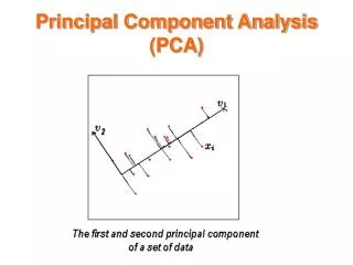
The first principal component (PC1) corresponds to the widest spread of the data. PC1 Spread along PC2 vector PC2 The next principal component (PC2) is perpendicular to the 1st, and corresponds to the next widest spread of the data. Spread along PC1 vector & so on. There will be as many PCs as data dimensions, but ranked by diminishing importance. http://web.media.mit.edu/~tristan/phd/dissertation/chapter5.html
Linear Transformations Scaling x2 X X a2x2 X X X X X X X X X O X X X O X X O X O O O O O O O O O O O O O O O O O x1 a1x1 Adapted from http://www.engr.sjsu.edu/~knapp/HCIRODPR/PR_Mahal/linear_tr.htm
Linear Transformations Scaling & Rotating x2 X X a21x1 + a22x2 X X X X X X X X X X X O X O X X O X O O O O O O O O O O O O O O O O O x1 a11x1 + a12x2 If we can stretch & rotate this way… Adapted from http://www.engr.sjsu.edu/~knapp/HCIRODPR/PR_Mahal/linear_tr.htm
Linear Transformations Scaling & Rotating x2 X X a21x1 + a22x2 X X X X X X X X X X X O X O X X O X O O O O O O O O O O O O O O O O O a11x1 + a12x2 x1 ...then we can also go the other way. To do this, we need to learn about covariance… Adapted from http://www.engr.sjsu.edu/~knapp/HCIRODPR/PR_Mahal/linear_tr.htm
More examples of different linear transformations: http://isomorphismes.tumblr.com/post/11407834056/matrices-linear-algebra
Covariance = measures tendency to vary together (to co-vary). Similar to correlation. xj xj xj xj xj X X X X X X X X X X X X X X X X xi xi xi xi xi X X X X X X X X X X X X X X X X X X X X X X X X c = -sisj c = -0.5 sisj c = 0 c = 0.5 sisj c = sisj Anti-correlated Uncorrelated Correlated Variance = average of the squared deviations of a feature from its mean = μ2 = (std deviation)2 = covar(i,i) Covariance = average of the products of the deviations of feature values from their means covar(i,j) = [ x(1,i) - m(i) ] [ x(1,j) - m(j) ] + ... + [ x(n,i) - m(i) ] [ x(n,j) - m(j) ] ( n - 1 ) Adapted from http://www.engr.sjsu.edu/~knapp/HCIRODPR/PR_Mahal/cov.htm
All of the covariances c(i,j) between features can be collected together into a covariance matrix C. This summarizes all of the correlation structure among all pairs of features. covariance between feature 1 and 2 covariance between feature 2 and n . . . c(1,2) c(1,n) c(1,1) . . . c(2,1) c(2,2) c(2,n) etc. C = . . . . . . . . . . . . c(n,1) c(n,n) c(n,2)
We need one last concept: Eigenvectors and eigenvalues The blue arrow is an eigenvector of this linear transformation matrix, since it doesn’t change direction. Its scale is also unchanged, so its eigenvalue is 1. Wikipedia
Calculating the PCA 1. Calculate the covariation matrix C between features of the data 2. Calculate the eigenvectors and eigenvalues of C 3. Order the eigenvectors according to the eigenvalues PC1 is the eigenvector corresponding to the largest eigenvalue, PC2 is the eigenvector corresponding to the next largest, etc. The data can be plotted as projections along the PCs of interest. genes PCs PCA patients patients mRNA abundances mRNA abundances Linear combinations of gene features All orthogonal Ranked from most important to least Now:
Here’s a beautiful application of PCA that illustrates how it can simplify complicated datasets: Men … 1 3000 1 What do you think are the most important genetic trends among European men? What might this picture look like? Table of SNPs Genotype ~3,000 European men (measure ~500K SNPs each using DNA microarrays) … SNPs … Calculate the most important “trends” in the data using Principal Component Analysis 500,000 PCA Visualize their genetic relationships by plotting each man as a point in “genotype space”, emphasizing only the most dominant genetic trends Plot of main genetic trends among European men
This is a map of their DNA. It recapitulates the map of Europe. In other words, the strongest genetic trends across European men relate directly to their geographic locations (note: not nationality)
Why? Genetic similarity is strongly distance dependent in Europe, presumably because people tend to live near where they were born and tend to marry locally.
The trend is so strong that it can be used to predict where the men are from, e.g. shown here by leave-one-out cross-validation:
SUMMARY In a sense, PCA fits a (multidimensional) ellipsoid to the data • Described by directions and lengths of principal (semi-)axes, e.g. the axis of a cigar or egg or the plane of a pancake encyclopedia2.thefreedictionary.com • No matter how an ellipsoid is turned, the eigenvectors point in those principal directions. The eigenvalues give the lengths. • The biggest eigenvalues correspond to the fattest directions (having the most data variance). The smallest eigenvalues correspond to the thinnest directions (least data variance). • Ignoring the smallest directions (i.e., collapsing them) loses relatively little information. Adapted from whuber, http://stats.stackexchange.com/questions/2691/making-sense-of-principal-component-analysis-eigenvectors-eigenvalues