Face Recognition using PCA (Eigenfaces) and LDA (Fisherfaces)
190 likes | 807 Vues
Face Recognition using PCA (Eigenfaces) and LDA (Fisherfaces). Pradeep Buddharaju. COSC 6397. U of H. Principal Component Analysis. A N x N pixel image of a face, represented as a vector occupies a single point in N 2 -dimensional image space.

Face Recognition using PCA (Eigenfaces) and LDA (Fisherfaces)
E N D
Presentation Transcript
Face Recognition using PCA (Eigenfaces) and LDA (Fisherfaces) Pradeep Buddharaju COSC 6397 U of H
Principal Component Analysis • A N x N pixel image of a face, represented as a vector occupies a single point in N2-dimensional image space. • Images of faces being similar in overall configuration, will not be randomly distributed in this huge image space. • Therefore, they can be described by a low dimensional subspace. • Main idea of PCA (cutler96): • To find vectors that best account for variation of face images in entire image space. • These vectors are called eigen vectors. • Construct a face space and project the images into this face space (eigenfaces).
Image Representation • Training set of images of size N*N are represented by vectors of size N2 1,2,3,…,M Example
Average Image and Difference Images • The average training set is defined by Ψ = (1/M) ∑Mi=1i • Each face differs from the average by vector Φi = Γi – Ψ
Covariance Matrix • A covariance matrix is constructed as: C = AAT, where A=[Φ1,…,ΦM] of size N2x N2 • Finding eigenvectors of N2x N2 matrix is intractable. Hence, use the matrix ATA of size M x M and find eigenvectors of this small matrix. Size of this matrix is N2 x N2 Size of this matrix is M*M
Eigenvalues and Eigenvectors - Definition • If v is a nonzero vector and λ is a number such that Av = λv, then v is said to be an eigenvector of A with eigenvalue λ. Example l (eigenvalues) (eigenvectors) A v
Eigenvectors of Covariance Matrix • The eigenvectors vi of ATA are: • Consider the eigenvectors vi of ATA such that • ATAvi = ivi • Premultiplying both sides by A, we have • AAT(Avi) = i(Avi)
Face Space • The eigenvectors of covariance matrix are ui = Avi Face Space • ui resemble facial images which look ghostly, hence called eigenfaces
Projection into Face Space • A face image can be projected into this face space by Ωk = UT(Γk – Ψ); k=1,…,M Projection of Image1
Recognition • The test image, Γ, is projected into the face space to obtain a vector, Ω: Ω = UT(Γ – Ψ) • The distance of Ω to each face class is defined by Єk2 = ||Ω-Ωk||2; k = 1,…,M • A distance threshold,Өc, is half the largest distance between any two face images: Өc = ½ maxj,k {||Ωj-Ωk||}; j,k = 1,…,M
Recognition • Find the distance, Є , between the original image, Γ, and its reconstructed image from the eigenface space, Γf, Є2 = || Γ – Γf ||2 , where Γf = U * Ω + Ψ • Recognition process: • IF Є≥Өcthen input image is not a face image; • IF Є<ӨcAND Єk≥Өc for all k then input image contains an unknown face; • IF Є<Өc AND Єk*=mink{ Єk} < Өcthen input image contains the face of individual k*
Limitations of Eigenfaces Approach • Variations in lighting conditions • Different lighting conditions for enrolment and query. • Bright light causing image saturation. • Differences in pose – Head orientation • - 2D feature distances appear to distort. • Expression • - Change in feature location and shape.
Linear Discriminant Analysis • PCA does not use class information • PCA projections are optimal for reconstruction from a low dimensional basis, they may not be optimal from a discrimination standpoint. • LDA is an enhancement to PCA • Constructs a discriminant subspace that minimizes the scatter between images of same class and maximizes the scatter between different class images
Mean Images • Let X1, X2,…, Xc be the face classes in the database and let each face class Xi, i = 1,2,…,c has k facial images xj, j=1,2,…,k. • We compute the mean image i of each class Xi as: • Now, the mean image of all the classes in the database can be calculated as:
Scatter Matrices • We calculate within-class scatter matrix as: • We calculate the between-class scatter matrix as:
Projection • We find the product of SW-1 and SB and then compute the Eigen vectors of this product (SW-1. SB). • Use same technique as eigenfaces approach to reduce the dimensionality of scatter matrix to compute eigenvectors. • Form a matrix U that represents all eigenvectors of SW-1. SB by placing each eigenvector ui as each column in that matrix. • Each face image xj Xi can be projected into this face space by the operation Ωi = UT(xj – )
Testing • Same as Eigenfaces Approach
References • Turk, M., Pentland, A.: Eigenfaces for recognition. J. Cognitive Neuroscience 3 (1991) 71–86 • Belhumeur, P., P.Hespanha, J., Kriegman, D.: Eigenfaces vs. fisherfaces: recognition using class specific linear projection. IEEE Transactions on Pattern Analysis and Machine Intelligence 19 (1997) 711–720