Download
1 / 36
360 likes | 396 Vues
This study explores the use of wavelet tools, such as Continuous Wavelet Transform and Discrete Wavelet Transform, to estimate trends in atmospheric data. Learn about wavelet properties, multiscale analysis, and the application of wavelet variance for assessing changes over time. Discover how wavelet coefficients provide insights into energy variations at different scales. Examples include the analysis of coral data and Nile river annual minima. The decorrelation properties of wavelet transform and the wavelet variance decomposition are also discussed. Explore the evaluation of trend detection and significance testing using wavelet analysis techniques.

E N D
NRCSE Using wavelet tools to estimate and assess trends in atmospheric data
Wavelets • Fourier analysis uses big waves • Wavelets are small waves
Requirements for wavelets • Integrate to zero • Square integrate to one • Measure variation in local averages • Describe how time series evolve in time for different scales (hour, year,...) • or how images change from one place to the next on different scales (m2, continents,...)
Continuous wavelets • Consider a time series x(t). For a scale l and time t, look at the average • How much do averages change over time?
Haar wavelet • where
Continuous Wavelet Transform • Haar CWT: • Same for other wavelets • where
Basic facts • CWT is equivalent to x: • CWT decomposes energy: energy
Discrete time • Observe samples from x(t): x0,x1,...,xN-1Discrete wavelet transform (DWT) slices through CWT • restricted to dyadic scales tj = 2j-1, j = 1,...,J t restricted to integers 0,1,...,N-1 Yields wavelet coefficients Think of as the rough of the series, so is the smooth (also called the scaling filter). A multiscale analysis shows the wavelet coefficients for each scale, and the smooth.
Properties • Let Wj = (Wj,0,...,Wj,N-1); S = (s0,...,sN-1). • Then W = (W1,...,WJ,S ) is the DWT of X = (x0,...,xN-1). • (1) We can recover X perfectly from its DWT W, X = W-1W. • (2) The energy in X is preserved in its DWT:
The pyramid scheme • Recursive calculation of wavelet coefficients: {hl } wavelet filter of even length L; {gl = (-1)lhL-1-l} scaling filter • Let S0,t = xt for each t • For j=1,...,J calculate • t = 0,...,N 2-j-1
Oxygen isotope in coral cores at Malindi, Kenya • Cole et al. (Science, 2000): 194 yrs of monthly d18O-values in coral core. • Decreased oxygen corresponds to increased sea surface temperature • Decadal variability related to monsoon activity
Long term memory • A process has long term memory if the autocorrelation decays very slowly with lag • May still look stationary • Example: Fractionally differenced Gaussian process, has parameter d related to spectral decay • If the process is stationary
Decorrelation properties of wavelet transform • Periodogram values are approximately uncorrelated at Fourier frequencies for stationary processes (but not for long memory processes) • Wavelet coefficient at different scales are also approximately uncorrelated, even for long memory processes (approximation better for larger L)
Nile river 1 yr 2 yr 4 yr 8 yr ≥16 yr
Wavelet variance • The wavelet coefficients pick up changes in the energy at different scales over time • The variability of the coefficients at each scale is a variance decomposition (similar to Fourier analysis, although the frequency choices are different) • The wavelet coefficients, even for a long-term memory process, behave (at each scale) like a sample from a mean zero white noise process (at least for large L)
Analysis of wavelet variance • In the Nile data there is a visual indication that the variability is changing after the first 100 observations at scales 1 and 2 years. • Let Xt be a time series with mean 0 and variance .To test • against • we use the statistics
Testing for changepoint of variability • Let and • D=max(D+,D-) measures the deviation of Kk from the 45° line expected if H0 is true. • Asymptotically, D converges to a Brownian bridge, which can be used to calculate critical values. • Alternatively Monte Carlo critical values, or simply Monte Carlo test.
Why did it change? • Around 715 a nilometer was constructed and located at a mosque on Rawdah Island in the river. Replaced 850 after a huge flood.
What is a trend? • “The essential idea of trend is that it shall be smooth” (Kendall,1973) • Trend is due to non-stochastic mechanisms, typically modeled independently of the stochastic portion of the series: • Xt = Tt + Yt
Wavelet analysis of trend • where A is diagonal, picks out S and the boundary wavelet coefficients. • Write • where R=WTAW, so if X is Gaussian we have
Confidence band calculation • Let v be the vector of sd’s of • and . Then • which we can make 1- by choosing d by Monte Carlo (simulating the distribution of U). • Note that this confidence band will be simultaneous, not pointwise.
Air turbulence • EPIC: East Pacific Investigation of Climate Processes in the Coupled Ocean-Atmosphere System • Objectives: (1) To observe and understand the ocean-atmosphere processes involved in large-scale atmospheric heating gradients • (2) To observe and understand the dynamical, radiative, and microphysical properties of the extensive boundary layer cloud decks
Flights • Measure temperature, pressure, humidity, air flow in East Pacific
Flight pattern • The airplane flies some high legs (1500 m) and some low legs (30 m). The transition between these (somewhat stationary) legs is of main interest in studying boundary layer turbulence.
Wavelet variability • The variability at each scale constitutes an analysis of variance. • One can clearly distinguish turbulent and non-turbulent regions.