Download
1 / 40
400 likes | 435 Vues
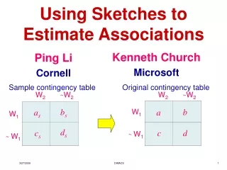
Using Sketches to Estimate Associations. Ping Li Cornell. Kenneth Church Microsoft. Sample contingency table. Original contingency table. W 2. ~ W 2. W 2. ~ W 2. b s. b. a s. W 1. a. W 1. d s. c s. c. d. ~ W 1. ~ W 1. Ken Church Albert Greenberg James Hamilton

E N D
Using Sketches to Estimate Associations Ping Li Cornell Kenneth Church Microsoft Sample contingency table Original contingency table W2 ~W2 W2 ~W2 bs b as W1 a W1 ds cs c d ~W1 ~W1 DIMACS
Ken Church Albert Greenberg James Hamilton {church, albert, jamesrh}@microsoft.com On Delivering Embarrassingly Distributed Cloud ServicesHotnets-2008 Board Affordable $1B $2M 2 DIMACS
Containers:Disruptive Technology Implications for Shipping New Ships, Ports, Unions Implications for Hotnets New Data Center Designs Power/Networking Trade-offs Cost Models: Expense vs. Capital Apps: Embarrassingly Distributed Restriction on Embarrassingly Parallel Machine Models: Distributed Parallel Cluster Parallel Cluster 3 DIMACS
Mega vs. Micro Data Centers 4 DIMACS
Related Work 220 containers in one PoP 220 in 220 PoPs 5 • http://en.wikipedia.org/wiki/Data_center • A data center can occupy one room of a building… • Servers differ greatly in size from 1U servers to large … silos • Very large data centers may use shipping containers...[2] DIMACS
Embarrassingly Distributed Probes • W1 & W2 are Shipping Containers • Lots of bandwidth within a container • But less across containers • Limited Bandwidth Sampling Sample contingency table Original contingency table W2 ~W2 W2 ~W2 bs b as W1 a W1 ds cs c d ~W1 ~W1 DIMACS
≈ 1990 Strong: 427M (Google) Powerful: 353M (Google) Page Hits ≈ 1000x BNC freqs DIMACS
PMI + The Web: Better together Turney (and Know It All) DIMACS
“It never pays to think until you’ve run out of data” – Eric Brill Moore’s Law Constant: Data Collection Rates Improvement Rates Banko & Brill: Mitigating the Paucity-of-Data Problem (HLT 2001) No consistently best learner More data is better data! Quoted out of context Fire everybody and spend the money on data DIMACS
# of (English) documents D≈ 1010 . Lots of hits even for very rare words. Larger corpora Larger counts More signal Page Hits Estimatesby MSN and Google(August 2005) More Freq Less Freq DIMACS
Joint frequencies ought to decrease monotonically as we add more terms to the query. Caution: Estimates ≠ Actuals These are just (quick-and-dirty) estimates (not actuals) DIMACS
Rule of Thumb breaks down when there are strong interactions (Common for cases of most interest) Query Planning (Governator): Rule of Thumb DIMACS
= = = + + f D f a a+b+c+d a b c 1 2 Associations: PMI, MI, Cos, R, Cor…Summaries of Contingency Table W2 ~W2 a: # of documents that contain both WordW1and WordW2 b W1 a b: # of documents that contain WordW1but not WordW2 c ~W1 d Margins (aka doc freq) • Need just one more constraint • To compute table (& summaries) • 4 parameters: a, b, c, d • 3 constraints: f1, f2, D DIMACS
Postings Margins (and more)(Postings aka Inverted File) Postings(w): A sorted list of doc IDs for w … This pig is so cute … … saw a flying pig … … was raining pigs and eggs … Doc #13 Doc #25 Doc #33 Assume doc IDs are random DIMACS
Conventional Random Sampling(Over Documents) Sample contingency table Original contingency table W2 ~W2 W2 ~W2 bs b as W1 a W1 ds cs c d ~W1 ~W1 Margin-Free Baseline Sample Size DIMACS
Random Sampling • Over documents • Simple & well understood • But problematic for rare events • Over postings • where f = |P| (P = postings, aka inverted file) • aka doc freq or margin Undesirable DIMACS
W2 ~W2 bs as Sketches >> Random Samples W1 ds cs ~W1 Best Undesirable Better DIMACS
Outline • Review random sampling • and introduce a running example • Sample: Sketches • A generalization of Broder’s Original Method • Sketches: • Advantages: Larger as than random sampling • Disadvantages: Estimation more challenging • Estimation: Maximum Likelihood (MLE) • Evaluation DIMACS
Random Sampling over Documents W2 ~W2 bs as W1 ds cs ~W1 • Doc IDs are random integers between 1 and D=36 • Small circles word W1 • Smallsquares word W2 • Choose a sample size: Ds = 18. Sampling rate = Ds/D = 50% • Construct sample contingency table: • as = #|{4,15}| = 2, bs = #|{3, 7, 9, 10, 18}| = 5, • cs= #|{2,5,8}| = 3, ds = #|{1,6,11,12,13,14,17}|= 8 • Estimation: a ≈ D/Ds as • But that doesn’t take advantage of margins DIMACS
Proposed Sketches Sketch = Front of Postings Postings P1: 3 4 7 9 10 15 18 19 24 25 28 33 P2: 2 4 5 8 15 19 21 24 27 28 31 35 Throw out red Choose sample size: Ds = 18 = min(18, 21) as = |{4,15}| = 2 bs = 7 – as = 5 cs= 5 – as = 3 ds = Ds–as–bs–cs= 8 W2 ~W2 Based on blue − red bs as W1 ds cs ~W1 DIMACS
When we know the margins, We ought to use them Estimation: Maximum Likelihood (MLE) • Consider all possible contingency tables: • a, b, c & d • Select the table that maximizes the probability of observations • as, bs, cs& ds DIMACS
Problem: Too complicated. Numerical problems. Exact MLE First derivative of log likelihood gives the MLE solution DIMACS
Log likelihood function is concave unique maximum Suffice to solve g(a) = 1. Exact MLE Second derivative: PMF updating formula: DIMACS
is a cubic function of a. Exact MLE MLE solution: DIMACS
P(as,bs; a) P(as,cs; a) Approximate MLE: Maximize P(as, bs, cs; a)=P(as, bs; a)×P(as,cs; a) An Approximate MLE Suppose we were sampling from the two inverted files directly and independently. DIMACS
An Approximate MLE Convenient Closed-Form Solution • Convenient Closed-Form • Surprisingly accurate • Recommended Take log of both sides; Set derivative = 0 DIMACS
Independence Baseline Evaluation Margin-Free Baseline When we know the margins, We ought to use them Proposed Best DIMACS
Theoretical Evaluation • Not surprisingly, there is a trade-off between • Computational work: space, time • Statistical Accuracy: variance, error • Formulas state trade-off precisely in terms of sampling rate: Ds/D • Theoretical evaluation: • Proposed MLE is better than Margin Free baseline • Confirms empirical evaluation DIMACS
At web scale (D≈1010), sampling rate 10- 4 may suffice for “ordinary” words. How many samples are enough? Sampling rate to achieve cv = SE/a < 0.5 Larger D Smaller sampling rate Cluster of 10k machines A Single machine DIMACS
Broder’s Sketch: Original & MinwiseEstimate Resemblance (R) • Notation • Words: w1, w2 • Postings: P1, P2 • Set of doc IDs • Resemblance: R • Random Permutation: π • Minwise Sketch: • Permute doc IDs k times: πk • For each πi,let mini(P) be smallest doc ID in πi(P) • Original Sketch: • Sketches: K1, K2 • Set of doc IDs • (front of postings) • Permute doc IDs once: π • Let K=firstk(P) be the first k doc IDs in π(P) Throw out half DIMACS
Degree of freedom = 2m – (m+1), increases exponentially, suggesting margin constraints become less important as m increases. Multi-way Associations: Evaluation MSE relative improvement over margin-free baseline When we know the margins, we ought to use them Gains are larger for 2-way than multi-way DIMACS
Conclusions (1 of 2) When we know the margins, We ought to use them • Estimating Contingency Tables: • Fundamental Problem • Practical app: • Estimating Page Hits for two or more words (Governator) • Know It All: Estimating Mutual Information from Page Hits • Baselines: • Independence: Ignore interactions (Awful) • Margin-Free: Ignore postings (Wasteful) • (≈2x) Broder’s Sketch (WWW 97, STOC 98, STOC 2002) • Throws out half the sample • (≈10x) Random Projections (ACL2005, STOC2002) • Proposed Method: • Sampling: like Broder’s Sketch, but throws out less • Larger as than random sampling • Estimation: MLE (Maximum Likelihood) • MF: Estimation is easy without margin constraints • MLE: Find most likely contingency table, • Given observations: as, bs, cs, ds DIMACS
Rising Tide of Data Lifts All BoatsIf you have a lot of data, then you don’t need a lot of methodology Conclusions (2 of 2) • Recommended Approximation • Trade-off between • Computational work (space and time) and • Statistical accuracy (variance and errors) • Derived formulas for variance • Showing how trade-off depends on sampling rate • At Web scales, sampling rate (Ds/D) 10–4 • A cluster of 10k machines A single machine DIMACS
Comparison with Broder’s Algorithm Broder’s Method has larger variance (≈2x) Because it uses only half the sketch Var(RMLE) << VAR(RB) Equal samples Proportional samples when DIMACS
Comparison with Broder’s Algorithm Ratio of variances (equal samples) Var(RMLE) << VAR(RB) DIMACS
Comparison with Broder’s Algorithm Ratio of variances (proportional samples) Var(RMLE) << VAR(RB) DIMACS
Comparison with Broder’s AlgorithmEstimation of Resemblance Broder’s method throws out half the samples 50% improvement DIMACS
Comparison with Random ProjectionsEstimation of Angle Huge Improvement DIMACS