Factorial ANOVAs
PSY 4603 Research Methods. Factorial ANOVAs. Here, we’ll consider experiments in which treatment conditions are classified with respect to the levels represented on two independent variables.


Factorial ANOVAs
E N D
Presentation Transcript
PSY 4603 Research Methods Factorial ANOVAs
Here, we’ll consider experiments in which treatment conditions are classified with respect to the levels represented on two independent variables. • In all these discussions, I will be assuming that subjects serve in only one of the treatment conditions, that they provide only a single score or observation, and that they are randomly assigned to one of the conditions. • We refer to these sorts of experiments as completely randomized factorial designs. • Iwill consider other types of designs later. • The most common means by which two or more independent variables are manipulated in an experiment is a factorial arrangement of the treatments or, more simply, a factorial experiment or design. • Iwill use these terms interchangeably.
Factorial designs are sometimes referred to as experiments in which the independent variables are completely crossed. • We can think of the crossing in terms of a multiplication of the levels of the different independent variables. • In this example, the treatment combinations may be enumerated by multiplying (small + medium + large) by (easy + hard) to produce the six treatment combinations of the design. • The factorial experiment is probably most effective at the reconstructive stage of science, where investigators begin to approximate the "real" world by manipulating a number of independent variables simultaneously. • It is clear, however, that the factorial experiment has advantages of economy, control, and generality. • Factorial designs are economical in the sense that they provide considerably more information than separate single factor experiments, often at reduced cost of subjects, time, and effort. • Factorial designs achieve experimental control by providing a way to remove important, but unwanted, sources of variability that otherwise would contribute to our estimates of error variance. • Finally, factorial designs allow us to assess the generality of a particular finding by studying the effects of one independent variable under different experimental conditions. • We evaluate this generality by examining the results of a factorial experiment for interactions. • We’ll discuss this concept again shortly.
A great deal of research in the business research consists of the identification of variables contributing to a given phenomenon. • Quite typically, an experiment may be designed to focus attention on a single independent variable or factor. • A main characteristic of this type of investigation is that it represents an assessment of how a variable operates under "ideal" conditions - with all other important variables held constant or permitted to vary randomly across the different conditions. • An alternative approach is to study the influence of one independent variable in conjunction with variations in one or more additional independent variables. • Here, the primary question is whether a particular variable studied concurrently with another variable in a factorial design will show the same effect as it would when studied separately in a single-factor (1 independent variable) design.
Basic Information AvailableFrom Factorial Designs • Factorial experiments are rich with information. • We can study not only the effects of the two independent variables separately but also how they combine to influence the dependent variable. • Simple Effects of an Independent Variable • A factorial design actually consists of a set of single-factor experiments. • Suppose we are putting together a technical reading series for our group of clients and that we have reason to believe that the format of the books will influence reading speed. • Two factors we might consider are the length of the printed lines and the contrast between the printed letters and the paper. • Let's assume that we chose three line lengths (3, 5, and 7 inches.) and three contrasts (low, medium, and high).
Suppose we created three single-factor experiments as follows: One consists of three groups of people randomly assigned to the different line conditions in which the letters for all three groups are printed with low contrast. • This single-factor experiment studies the effects of line length on reading speed under conditions of low contrast, and if the manipulation were successful, we would attribute any significant differences to the variation of line length. • Two other experiments are exact duplicates of the first except that the letters are printed with medium contrast for one and with high contrast for the other.
As you can see, these experiments represent component parts of a factorial design. • Each component experiment provides information about the effects of line length, but under different conditions of contrast.
As diagramed in the table, we can also view the factorial design as a set of component single-factor experiments involving the other independent variable, contrast. • The left-hand experiment at the top of the table consists of a single-factor design in which different groups of subjects receive the reading material under one of three conditions of contrast (low, medium, or high); all children read material printed in 3-inch lines. • The second experiment duplicates the first exactly except that the material is printed with 5-inch lines; similarly, the third duplicates the first except that the material is printed with 7-inch lines. Each component experiment provides information about the effects of contrast, but for lines of different length.
The results of these component single-factor experiments are called the simple effects of an independent variable.1 • 1They are more commonly called the simple main effects of an independent variable. I prefer to use • the shorter version (simple effects) to distinguish these effects from another statistical concept, namely, • main effects. I will consider this concept later.
Main Effects • The main effects of an independent variable refer to the average (mean of simple effects) of the component single-factor experiments making up the factorial design. • The main effect of line length, for example, refers to the effects of this independent variable when the other independent variable, contrast, is ignored or disregarded.
As illustrated by the arrows in Table 3, we obtain this main effect by combining the individual treatment means from each component experiment involving the manipulation of line length to produce new averages that reflect variations in line length alone. • In a similar fashion, we obtain the main effect of the contrast variable by combining the means from each component experiment involving the manipulation of contrast. • Main effects are most easily interpreted when interaction is absent. • Under these circumstances, the effects of either independent variable-line length or contrast - do not depend on the other independent variable, implying that we can safely combine these results and study the effects of each independent variable separately. • In the same way we would study the effects from two actual single-factor experiments, even though the data are combined from a factorial design.
Interaction Effects • Although it may be informative to study the effects of the two independent variables separately for each component single-factor experiment, we would certainly want to compare these results. • For example, we would want to determine whether the simple effects of line length that we find with low contrast are the same as those we observe for medium contrast or for high contrast. • Similarly, we would also want to know whether the simple effects of contrast that we obtain with 3-inch lines are the same as those we observe for 5- and 7-inch lines. • A unique feature of the factorial design is the possibility of comparing the results of each set of three component single-factor experiments, one involving the three line-length experiments and the other involving the three contrast experiments. • A comparison of this sort - a comparison among the simple effects of the component experiments is called the analysis of interaction. • If the outcomes of the different component experiments within either set are the same, interaction is absent; that is, if the effects of the component experiments are duplicated for each level of the other independent variable, there is no interaction. • On the other hand, if the outcomes are different, interaction is present: The effects of the component experiments are not the same for all levels of the other independent variable.
More on the Concept of Interaction • Interaction is the one new concept introduced by the factorial experiment. • Main effects have essentially the same meaning as in the single-factor analysis of variance and they are calculated in exactly the same way. • Moreover, as you will see in later, factorials with three or more variables involve no additional principles. • Thus, it is important to understand the single-factor analysis of variance since many of the principles and procedures found in this simplest of experimental designs - such as partitioning sums of squares, the logic of hypothesis testing, and planned and post hoc comparisons-are also found in the more complicated designs. • By the same token, the two-factor analysis of variance forms a building block for designs involving three or more variables, with the concept of interaction linking them all together.
An Example of No Interaction • The table below presents some hypothetical results for the experiment on reading speed. • Assume that equal numbers of adults are included in each of the nine conditions and that the values presented in the table represent the average reading scores found in the experiment.
I will refer to line length as factor A and to the three line lengths defining that independent variable as levels a1, a2, and a3. • Correspondingly, I will refer to contrast as factor B and to the three levels of contrast as levels b1, b2, and b3. • The main effect of line length (factor A) is obtained by summing (or collapsing over) the three cell means for the different contrast conditions and then averaging these sums. • The last row of the table gives these means for the three length conditions. • These averages are called the column marginal means of the matrix. • Thus, the average reading speed for subjects in the 3-inch condition is found by combining the means from the three contrast conditions and calculating an average. • In this case, we have: YA1 = .89 + 3.89 + 4.22 = 9.00 = 3.00 3 3 • This mean represents the average performance of all the subjects in the experiment who received the 3-inch lines; the specific conditions of factor B, namely, the three contrasts, are unimportant at this point. • We can obtain similar averages for the subjects receiving the 5- and 7-inch materials. • These two marginal means are given in the other two columns.
In a like fashion, the row marginal averages give us information concerning the main effect of the different contrasts. • That is, the average reading speed for subjects in the low-contrast condition is given by an average of the means for the three length conditions. Thus, YB1 = .89 + 2.22 + 2.89 = 6.00 = 2.00 3 3 • This averaging for the other contrast conditions appears in the final column of the table. • Each of these marginal means represents the average performance of all the subjects who received the specified contrast condition, disregarding the particular condition of factorial - that is, which line length-these subjects also received.
Let's look first at the marginal averages for line length, which are plotted on the left side in Figure 1. • As you can see, reading speed increases steadily as the length of the lines increases from 3 to 7 inches. • You can think of this plot as a general description of the overall or main effects of factorial.
Now, would you say that this overall relationship is representative of the results obtained in the component single-factor experiments found in the three rows within the body of the last table? • To help answer this question, I have plotted these cell means in a double classification plot on the right side of the Figure. • I accomplished this classification by marking off line length on the baseline, plotting the cell means on the graph, and connecting the means from the same component single-factor experiment. • It is clear that the functions for the three component experiments are parallel, which means that the pattern of differences obtained with line length is exactly the same at each level of the other independent variable. • There is no interaction!!
We arrive at the same conclusion if we focus on the other independent variable, contrast. • The left-hand graph in Figure 2 plots the main (or average) effects of factor B. • Low contrast produces the lowest reading scores, and medium and high contrast produce higher but similar averages.
In the absence of interaction, we usually focus our attention on the main effects - that is, the two sets of marginal means - rather than on the cell means. • Since the effects of line length, for example, do not depend on any particular condition of contrast, we can safely combine the results from the relevant component experiments without distorting the outcome of the experiment. • We can make a similar argument for the contrast variable.
The next table presents a second set of hypothetical results using the same experimental design. • Note that the same main effects are present; that is, the means in the row and column margins of the last table 5 are identical to the corresponding means in the margins of this one. • There is a big difference, however, when we look at the simple effects of the two independent variables.
In either plot, you can clearly see that the patterns of differences reflected by the simple effects are not the same at all levels of the other independent variable - interaction is present.
To be more specific, consider the simple effects of line length at level b1 - the cell means in the first row of the table. • This row is the component single-factor experiment in which all subjects are tested under conditions of low contrast. • These three means are plotted in the left-hand graph (below). • An inspection of the figure indicates that the relationship is positive and even linear. • The simple effect at level b2 (the second row) also shows a positive linear trend for all the subjects receiving the medium materials, although it is steeper than in the low-contrast case. • But see what happens to the subjects who receive the high-contrast materials. • The relationship in this third component experiment is curvilinear: • The reading scores first increase and then decrease with line length. • You can see an analogous deviation of the simple effects when we look at the cell means in each of the three data columns, which are plotted in the right-hand graph of the figure.
Here, we are considering the component experiments in which contrast is varied while length is held constant. • For the simple effect of contrast for 3-inch lines (the first column), you can see that the relationship is linear. • For the simple effect for 5-inch lines (the second column), the relationship is not as sharply defined, with the function starting to "bend over" away from the linear trend. • In the third column (7-inch lines), we have an actual reversal of the trend-that is, a curvilinear relationship, maximum performance being found with a medium contrast. • With either plot of the data, then, we can determine at a glance that the particular form of the relationship between the independent variable plotted against the baseline (line length or contrast) and the scores-that is, the shape of the curve drawn between successive points on the baseline-is not the same at the three different levels of the other independent variable. • A simple way to describe this situation is to say that the three curves are not parallel.
So, the main effects are not representative of the simple effects and, thus, provide a distorted view of the actual outcome of the single-factor experiments making up the factorial design. • There was no such distortion with our first example in which the interaction was absent.
Defining Interaction • The presence of interaction indicates that conclusions based on main effects alone will not fully describe the outcome of a factorial experiment. • Instead, the effects of each independent variable must be interpreted with the levels of the other independent variable in mind. • One definition is stated in terms of the two independent variables: An interaction is present when the effects of one independent variable on behavior change at the different levels of the second independent variable. • This definition contains a critical point often missed by beginning students, namely, the focus on the behavioral effects of the independent variables. • A common mistake is to think of two independent variables as influencing one another. • One independent variable does not influence the other independent variable-this makes no sense-yet students often make this mistake on an examination. • Independent variables influence the dependent variable, the behavior under study in an experiment.
Another way of defining interaction is to focus on the pattern of results associated with an independent variable. That is, An interaction is present when the pattern of differences associated with an independent variable changes at the different levels of the other independent variable. • The pattern of differences refers to the analysis of the effects of a complex, multilevel factor into a number of meaningful single-df comparisons-that is, differences between means. • Each component single-factor experiment, which makes up a factorial design, may be analyzed with these comparisons in mind. Suppose, for example, one of the independent variables consists of three levels, a control and two experimental treatments. • We would probably consider examining a number of differences between two means, such as a comparison between the two experimental treatments, a comparison between the control and each of the experimental treatments, and a comparison between the control and the combined experimental treatments. • If an interaction is present, the specific pattern of these differences will not all be the same for each of the component single-factor experiments constituting the factorial. • We will consider analyses that focus on these patterns of differences later. • Finally, a moreformal definition of interaction is in terms of the simple effects since a simple effect is the effect of one independent variable at a specific level of the other independent variable: An interaction is present when the simple effects of one independent variableare not the same at all levels of the second independent variable.
Graphical description of all possible relationships between factors A and B.
Analytic Concerns (With Graphs) • Generally, four types of graphs can result from graphing the cell means in two-way ANOVAs, as shown in the following figures • Of most concern to the researcher are graphs 5, 6, and 7. • When there are a significant effect and a main effect present in a study, the researcher must examine the interaction carefully before interpreting the main effect. • Often, there is little interest in comparisons among means for main effects.
When examining a two-way ANOVA, what should you do? (1) The presence of interaction always calls for an examination of the main effects and the data itself. (2) The presence of interaction may be important in and of itself if the purpose of the analysis is to test the significance of the interaction. • The purpose of the next example study was to test the combined effects of company size and age of executive on attitude. • As we’ll see, the interaction is significant at = 0.05. Also, the B effect is significant. Because we are not concerned with the B effects, we need only interpret the interaction.
As can be seen a bit later, the simple main effects of B are not the same at different levels of A. Simply, this is interpreted as follows: • In smaller companies, younger executives have more favorable attitudes toward economic policy, whereas in larger companies, the older executives have a more favorable attitude.
Warnings Post hoc tests are not performed for AGE because there are fewer than three groups.
Order of Significance Tests: The bottom line is this. When assessing your data, start with higher order interactions first. If they are significant, decompose the interaction(s). If not, go to lower order interactions followed by main effects. I recommend, as do others, not to include more than 4 independent variables at one time. Anything above this is just too cumbersome.
Multiple Comparisons • When the null hypothesis is rejected, it may be desirable to find which mean(s) is (are) different, and at what ranking order. • Many statistical inference procedures, geared at doing this, are possible; here are three: • Fisher’s least significant difference (LSD) method • Bonferroni adjustment • Tukey’s multiple comparison method