Download

1 / 54
560 likes | 694 Vues
This guide explores the fundamental concepts of statistical tests, specifically Z-Tests, T-Tests, and ANOVAs, providing insight into their application in predicting the future from samples. It covers key ideas such as null and alternative hypotheses, P-values, type errors, and interpretation of results. By using examples like brain volume changes after childbirth, it illustrates how these tests help researchers make informed conclusions about population effects. The document emphasizes the importance of statistical significance and correlation in understanding variable relationships.

E N D
T Tests and ANovas Jennifer Siegel
Objectives Statistical background Z-Test T-Test Anovas
Predicting the Future from a Sample • Science tries to predict the future • Genuine effect? • Attempt to strengthen predictions with stats • Use P-Value to indicate our level of certainty that result = genuine effect on whole population (more on this later…)
The Basics • Develop an experimental hypothesis • H0 = null hypothesis • H1 = alternative hypothesis • Statistically significant result • P Value = .05
P-Value • Probability that observed result is true • Level = .05 or 5% • 95% certain our experimental effect is genuine
Errors! • Type 1 = false positive • Type 2 = false negative • P = 1 – Probability of Type 1 error
Research Question Example • Let’s pretend you came up with the following theory… Having a baby increases brain volume (associated with possible structural changes)
Populations versus Samples Z - test T - test
Z-Test • Population
Some Problems with a Population-Based Study • Cost • Not able to include everyone • Too time consuming • Ethical right to privacy Realistically researchers can only do sample based studies
T-Test • T = differences between sample means / standard error of sample means • Degrees of freedom = sample size - 1
Hypothesise • H0 = There is no difference in brain size before or after giving birth • H1 = The brain is significantly smaller or significantly larger after giving birth (difference detected)
Absolute Brain Volumes cm3 T=(1271-1236)/(119-113)
Results: p=.003 Women have a significantly larger brain after giving birth http://www.danielsoper.com/statcalc/calc08.aspx
Types of T-Tests One-sample (sample vs. hypothesized mean) Independent groups (2 separate groups) Repeated measures (same group, different measure)
ANOVA • ANalysis Of VAriance • Factor = what is being compared (type of pregnancy) • Levels = different elements of a factor (age of mother) • F-Statistic • Post hoc testing
Different types of Anova • 1 Way Anova • 1 factor with more than 2 levels • Factorial Anova • More than 1 factor • Mixed Design Anovas • Some factors are independent, others are related
What can be concluded from ANOVA • There is a significant difference somewhere between groups • NOT where the difference lies • Finding exactly where the difference lies requires further statistical analysis = post hoc analysis
Conclusions • Z-Tests for populations • T-Tests for samples • ANOVAS compare more than 2 groups in more complicated scenarios
Correlation and Linear Regression VarunV.Sethi
Objective Correlation Linear Regression Take Home Points.
Correlation - How much linear is the relationship of two variables? (descriptive) Regression - How good is a linear model to explain my data? (inferential)
Correlation Correlation reflects the noisiness and direction of a linear relationship (top row), but not the slope of that relationship (middle), nor many aspects of nonlinear relationships (bottom).
Y Y Y Y Y Y X X Positive correlation Negative correlation No correlation Correlation • Strength and direction of the relationship between variables • Scattergrams
Measures of Correlation • Covariance • 2) Pearson Correlation Coefficient (r)
1) Covariance • The covariance is a statistic representing the degree to which 2 variables vary together • {Note that Sx2 = cov(x,x) }
A statistic representing the degree to which 2 variables vary together • Covariance formula • cf. variance formula
2) Pearson correlation coefficient (r) • r is a kind of ‘normalised’ (dimensionless) covariance • r takes values fom -1 (perfect negative correlation) to 1 (perfect positive correlation). r=0 means no correlation (S = st dev of sample)
Pearson – ‘Strength of Linear Relation’ r = 0.816
Limitations: • Sensitive to extreme values • Relationship not a prediction. • Not Causality
Regression: Prediction of one variable from knowledge of one or more other variables
How good is a linear model (y=ax+b) to explain the relationship of two variables? • If there is such a relationship, we can ‘predict’ the value y for a given x. (25, 7.498)
Linear dependence between 2 variables Two variables are linearly dependent when the increase of one variable is proportional to the increase of the other one y x Samples: - Energy needed to boil water - Money needed to buy coffeepots
εi = ŷi, predicted = yi , observed εi = residual Fiting data to a straight line (o viceversa): • Here, ŷ = ax + b • ŷ : predicted value of y • a: slope of regression line • b: intercept ŷ = ax + b • Residual error (εi): Difference between obtained and predicted values of y (i.e. yi- ŷi) • Best fit line (values of b and a) is the one that minimises the sum of squared errors (SSerror) (yi- ŷi)2
Adjusting the straight line to data: • Minimise (yi- ŷi)2 , which is (yi-axi+b)2 • Minimum SSerror is at the bottom of the curve where the gradient is zero – and this can found with calculus • Take partial derivatives of (yi-axi-b)2 respect parametres a and b and solve for 0 as simultaneous equations, giving: • This can always be done
How good is the model? • We can calculate the regression line for any data, but how well does it fit the data? • Total variance = predicted variance + error variance sy2 = sŷ2 + ser2 • Also, it can be shown that r2 is the proportion of the variance in y that is explained by our regression model r2 = sŷ2 / sy2 • Insert r2 sy2 into sy2 = sŷ2 + ser2 and rearrange to get: ser2 = sy2 (1 – r2) From this we can see that the greater the correlation the smaller the error variance, so the better our prediction
Is the model significant? • Do we get a significantly better prediction of y from our regression equation than by just predicting the mean? F-statistic
Practical Uses of Linear Regression • Prediction / Forecasting • Quantify strength between y and Xj( X1, X2, X3 )
General Linear Model • A General Linear Model is just any model that describes the data in terms of a straight line • Linear regression is actually a form of the General Linear Model where the parameters are b, the slope of the line, and a, the intercept. y = bx + a +ε