T-Tests for Statistical Analysis
Explore the fundamentals of T-tests and hypothesis testing, including differences between T-tests and Z-tests, determining probabilities of T, conducting hypothesis tests, and reporting results in research papers.


T-Tests for Statistical Analysis
E N D
Presentation Transcript
T-Tests Lecture: Nov. 6, 2002
Review • So far we have learned how to test hypothesis for two types of data: • Binomial data using the binomial distribution (test statistic: p) • Comparison of a sample mean to a known population mean and variance. (test statistic: z)
T-Tests • Z-tests require that we know the population standard deviation, which is often NOT known. • In these cases, we have to use the sample variance and standard deviation, as estimates of the population variance and standard deviation.
T-Tests • Population standard error (sX)=s2 / n • Use sample variance (df = N – 1) • Sample standard error (sX)= s2 / n • This creates a new statistic, the t statistic. • t = X – m / sX
T-Tests • The only difference between a t-test and a z-test is the use of sample variance, not population variance in the formula. • The degrees of freedom for a t-test is N-1. • The greater the degrees of freedom (i.e., the greater the N), the more accurate the t-statistic represents the z-score.
T-tests and Distributions • Each statistic has an underlying distribution. • Binomial p = binomial distribution which changes depending on p, N, and r. • z-scores = normal distribution • t-statistics = t-distribution • Changes depending on the degrees of freedom. • Larger the degrees of freedom, the more it approximates the normal distribution.
T-statistics and Distributions • The t distribution is bell-shaped, but more spread out. • Greater the N, and, thus, the degrees of freedom, the less spread out the t distribution.
Determining Probabilities of t • Just as you look up the probability of obtaining a z score using the unit normal table, we simply look up given t-statistic using a table for the t distribution (page 693 in textbook). • However, we must also know the degrees of freedom.
Hypothesis Testing with the t-test Example: A researcher knows that in 1990 the average age at which 25-year-olds report having their first drink was 16. The researcher predicts that that ten years later, 25-year-olds would report a significantly younger first age of drinking. She recruits 20 25-year-olds for her study and asks when each participant had his/her first drink.
Hypothesis Testing with the t-test • First she constructs her hypotheses. H0: mage of first drink = 16 Ha: mage of first drink = 16
Hypothesis Testing with the t-test • Create a decision rule. • Set the alpha level; a = .05. • Find the “critical t” in on our t-table. • Because non-directional hypothesis, we must find t-value that for which that t-value or higher is < .05 using two-tails. • Must look up based on 19 degrees of freedom (N – 1). • This t-statistic is 2.093. • So, if we get a t-statistic > 2.086, we can reject the null hypothesis.
Hypothesis Testing with the t-test • Collect data and calculate a t-statistic. • Assume researcher found that in her sample of 20 adults, the average age of first drink was 14, and the variance of 4. • The standard error of the t-statistic. s2/n = 4/20 = .45 The t-statistic is: X – m / sX = 14-16/.45 = -2/.45 = - 4.44
Hypothesis Testing with the t-test • Apply the decision rule. • Is our obtained t-statistic equal to or larger than our “critical t”? • Obtained t: -4.44 • Critical t: 2.093 • The absolute value of our t-statistic is more extreme. In other words, there is less than a 5% probability that if the population mean is 16 that we would obtain a sample mean of 14 with a variance of 4. • Reject the null hypothesis; accept the alternative hypothesis.
Assumptions of the t-test • All observations must be independent. • The population distribution of scores must be normally distributed.
Reporting a t-test • When reporting a t-statistic you should provide the sample mean and sample standard deviation somewhere in the paper. • You should also report the t-statistic, the degrees of freedom, whether it fell within the region of rejection, and whether it was a one- or two-tailed test.
Reporting a t-test Example: The 20 participants reported the age at which they had their first drink (M = 14, SD = 2). This age was significantly different from the average age of 16 reported a decade earlier, t(19) = -4.44, p < .05, two-tailed.