The t Tests
The t Tests. Single Sample Dependent Samples Independent Samples. From Z to t …. In a Z test, you compare your sample to a known population, with a known mean and standard deviation.

The t Tests
E N D
Presentation Transcript
The t Tests Single Sample Dependent Samples Independent Samples
From Z to t… • In a Z test, you compare your sample to a known population, with a known mean and standard deviation. • In real research practice, you often compare two or more groups of scores to each other, without any direct information about populations. • Nothing is known about the populations that the samples are supposed to come from.
The t Test for a Single Sample • The single sample t test is used to compare a single sample to a population with a known mean but an unknown variance. • The formula for the t statistic is similar in structure to the Z, except that the t statistic uses estimated standard error.
From Z to t… Note lowercase “s”.
Why (n – 1)? • To calculate the variance of a sample, when estimating the variance of its population, use (n -1) in order to provide an unbiased estimate of the population variance. • When you have scores from a particular group of people and you want to estimate what the variance would be for people in general who are like the ones you have scores from, use (n -1). Population of 1, 2, 3
Degrees of Freedom • The number you divide by (the number of scores minus 1) to get the estimated population variance is called the degrees of freedom. • The degrees of freedom is the number of scores in a sample that are “free to vary”.
Degrees of Freedom • Imagine a very simple situation in which the individual scores that make up a distribution are 3, 4, 5, 6, and 7. • If you are asked to tell what the first score is without having seen it, the best you could do is a wild guess, because the first score could be any number. • If you are told the first score (3) and then asked to give the second, it too could be any number.
Degrees of Freedom • The same is true of the third and fourth scores – each of them has complete “freedom” to vary. • But if you know those first four scores (3, 4, 5, and 6) and you know the mean of the distribution (5), then the last score can only be 7. • If, instead of the mean and 3, 4, 5, and 6, you were given the mean and 3, 5, 6, and 7, the missing score could only be 4.
Degrees of Freedom • In the t test, because the known sample mean is used to replace the unknown population mean in calculating the estimated standard deviation, one degree of freedom is lost. • For each parameter you estimate, you lose one degree of freedom. • Degrees of freedom is a measure of how much precision an estimate of variation has. • A general rule is that the degrees of freedom decrease when you have to estimate more parameters.
The t Distribution • In the Z test, when the population distribution follows a normal curve, the shape of the distribution of means will also be a normal curve. • However, this changes when you do hypothesis testing with an estimated population variance. • Since our estimate of is based on our sample… • And from sample to sample, our estimate of will change, or vary… • There is variation in our estimate of , and more variation in the t distribution.
The t Distribution • Just how much the t distribution differs from the normal curve depends on the degrees of freedom. • The t distribution differs most from the normal curve when the degrees of freedom are low (because the estimate of the population variance is based on a very small sample). • Most notably, when degrees of freedom is small, extremely large t ratios (either positive or negative) make up a larger-than-normal part of the distribution of samples.
The t Distribution • This slight difference in shape affects how extreme a score you need to reject the null hypothesis. • As always, to reject the null hypothesis, your sample mean has to be in an extreme section of the comparison distribution of means.
The t Distribution • However, if the distribution has more of its means in the tails than a normal curve would have, then the point where the rejection region begins has to be further out on the comparison distribution. • Thus, it takes a slightly more extreme sample mean to get a significant result when using a t distribution than when using a normal curve.
The t Distribution • For example, using the normal curve, 1.96 is the cut-off for a two-tailed test at the .05 level of significance. • On a t distribution with 3 degrees of freedom (a sample size of 4), the cutoff is 3.18 for a two-tailed test at the .05 level of significance. • If your estimate is based on a larger sample of 7, the cutoff is 2.45, a critical score closer to that for the normal curve.
The t Distribution • If your sample size is infinite, the t distribution is the same as the normal curve. http://www.econtools.com/jevons/java/Graphics2D/tDist.html
Since it takes into account the changing shape of the distribution as n increases, there is a separate curve for each sample size (or degrees of freedom). However, there is not enough space in the table to put all of the different probabilities corresponding to each possible t score. The t table lists commonly used critical regions (at popular alpha levels). The t Table
If your study has degrees of freedom that do not appear on the table, use the next smallest number of degrees of freedom. Just as in the normal curve table, the table makes no distinction between negative and positive values of t because the area falling above a given positive value of t is the same as the area falling below the same negative value. The t Table
The t Test for a Single Sample: Example You are a chicken farmer… if only you had paid more attention in school. Anyhow, you think that a new type of organic feed may lead to plumper chickens. As every chicken farmer knows, a fat chicken sells for more than a thin chicken, so you are excited. You know that a chicken on standard feed weighs, on average, 3 pounds. You feed a sample of 25 chickens the organic feed for several weeks. The average weight of a chicken on the new feed is 3.49 pounds with a standard deviation of 0.90 pounds. Should you switch to the organic feed? Use the .05 level of significance.
Hypothesis Testing • State the research question. • State the statistical hypothesis. • Set decision rule. • Calculate the test statistic. • Decide if result is significant. • Interpret result as it relates to your research question.
The t Test for a Single Sample: Example • State the research question. • Does organic feed lead to plumper chickens? • State the statistical hypothesis.
The t Test for a Single Sample: Example • Calculate the test statistic.
The t Test for a Single Sample: Example • Decide if result is significant. • Reject H0, 2.72 > 1.711 • Interpret result as it relates to your research question. • The organic feed caused the chickens to gain weight.
The t Test for a Single Sample: Example Odometers measure automobile mileage. How close to the truth is the number that is registered? Suppose 12 cars travel exactly 10 miles (measured beforehand) and the following mileage figures were recorded by the odometers: 9.8, 10.1, 10.3, 10.2, 9.9, 10.4, 10.0, 9.9, 10.3, 10.0, 10.1, 10.2 Using the .01 level of significance, determine if you can trust your odometer.
The t Test for a Single Sample: Example • State the research question. • Are odometers accurate? • State the statistical hypotheses.
The t Test for a Single Sample: Example • Set the decision rule.
The t Test for a Single Sample: Example • Calculate the test statistic. X2 96.04 102.01 106.09 104.04 98.01 108.16 100.00 98.01 106.09 100.00 102.01 104.04 1224.87 X 9.8 10.1 10.3 10.2 9.9 10.4 10.0 9.9 10.3 10.0 10.1 10.2 121.20
The t Test for a Single Sample: Example • Decide if result is significant. • Fail to reject H0, 1.25<3.106 • Interpret result as it relates to your research question. • The mileage your odometer records is not significantly different from the actual mileage your car travels.
The t Test for Dependent Samples • The t test for a single sample is for when you know the population mean but not its variance, and where you have a single sample of scores. • In most research, you do not even know the population’s mean. • And, in most research situations, you have not one set, but two sets of scores.
The t Test for Dependent Samples • Repeated-Measures Design • When you have two sets of scores from the same person in your sample, you have a repeated-measures, or within-subjects design. • You are more similar to yourself than you are to other people.
The t Test for Dependent Samples • Related-Measures Design • When each score in one sample is paired, on a one-to-one basis, with a single score in the other sample, you have a related-measures or matched samples design. • You use a related-measures design by matching pairs of different subjects in terms of some uncontrolled variable that appears to have a considerable impact on the dependent variable.
The t Test for Dependent Samples • You do a t test for dependent samples the same way you do a t test for a single sample, except that: • You use difference scores. • You assume the population mean is 0.
Difference Scores • The way to handle two scores per person, or a matched pair, is to make difference scores. • For each person, or each pair, you subtract one score from the other. • Once you have a difference score for each person, or pair, in the study, you treat the study as if there were a single sample of scores (scores that in this situation happen to be difference scores).
A Population of Difference Scores with a Mean of 0 • The null hypothesis in a repeated-measures design is that on the average there is no difference between the two groups of scores. • This is the same as saying that the mean of the population of the difference scores is 0.
The t Test for Dependent Samples: An Example • State the research hypothesis. • Does listening to a pro-socialized medicine lecture change an individual’s attitude toward socialized medicine? • State the statistical hypotheses.
The t Test for Dependent Samples: An Example • Set the decision rule.
The t Test for Dependent Samples: An Example • Calculate the test statistic.
The t Test for Dependent Samples: An Example • Decide if your results are significant. • Reject H0, -4.76<-2.365 • Interpret your results. • After the pro-socialized medicine lecture, individuals’ attitudes toward socialized medicine were significantly more positive than before the lecture.
The t Test for Dependent Samples: An Example At the Olympic level of competition, even the smallest factors can make the difference between winning and losing. For example, Pelton (1983) has shown that Olympic marksmen shoot much better if they fire between heartbeats, rather than squeezing the trigger during a heartbeat. The small vibration caused by a heartbeat seems to be sufficient to affect the marksman’s aim. The following hypothetical data demonstrate this phenomenon. A sample of 6 Olympic marksmen fires a series of rounds while a researcher records heartbeats. For each marksman, an accuracy score (out of 100) is recorded for shots fired during heartbeats and for shots fired between heartbeats. Do the data indicate a significant difference? Test with an alpha of .05. During Heartbeats Between Heartbeats 93 98 90 94 95 96 92 91 95 97 91 97
The t Test for Dependent Samples: An Example • State the research hypothesis. • Is better accuracy achieved by marksmen when firing the trigger between heartbeats than during a heartbeat? • State the statistical hypotheses.
The t Test for Dependent Samples: An Example • Set the decision rule.
The t Test for Dependent Samples: An Example • Calculate the test statistic. During Between Difference D2 93 98 -5 25 90 94 -4 16 95 96 -1 1 92 91 1 1 95 97 -2 4 91 97 -6 36 TOTAL -17 83
The t Test for Dependent Samples: An Example • Decide if your results are significant. • Reject H0, -2.62<-2.015 • Interpret your results. • Marksmen are significantly more accurate when they pull the trigger between heartbeats than during a heartbeat.
Issues with Repeated Measures Designs • Order effects. • Use counterbalancing in order to eliminate any potential bias in favor of one condition because most subjects happen to experience it first (order effects). • Randomly assign half of the subjects to experience the two conditions in a particular order. • Practice effects. • Do not repeat measurement if effects linger.
The t Test for Independent Samples • Observations in each sample are independent (not related to) each other. • We want to compare differences between sample means, not a mean of differences.
Sampling Distribution of the Difference Between Means • Imagine two sampling distributions of the mean... • And then subtracting one from the other… • If you create a sampling distribution of the difference between the means… • Given the null hypothesis, we expect the mean of the sampling distribution of differences, 1- 2, to be 0. • We must estimate the standard deviation of the sampling distribution of the difference between means.
Pooled Estimate of the Population Variance • Using the assumption of homogeneity of variance, both s1 and s2 are estimates of the same population variance. • If this is so, rather than make two separate estimates, each based on some small sample, it is preferable to combine the information from both samples and make a single pooled estimate of the population variance.
Pooled Estimate of the Population Variance • The pooled estimate of the population variance becomes the average of both sample variances, once adjusted for their degrees of freedom. • Multiplying each sample variance by its degrees of freedom ensures that the contribution of each sample variance is proportionate to its degrees of freedom. • You know you have made a mistake in calculating the pooled estimate of the variance if it does not come out between the two estimates. • You have also made a mistake if it does not come out closer to the estimate from the larger sample. • The degrees of freedom for the pooled estimate of the variance equals the sum of the two sample sizes minus two, or (n1-1) +(n2-1).