LECTURE 04: MAXIMUM LIKELIHOOD ESTIMATION
LECTURE 04: MAXIMUM LIKELIHOOD ESTIMATION. • Objectives: Discrete Features Maximum Likelihood Bias in ML Estimates Bayesian Estimation Example

LECTURE 04: MAXIMUM LIKELIHOOD ESTIMATION
E N D
Presentation Transcript
LECTURE 04: MAXIMUM LIKELIHOOD ESTIMATION • • Objectives:Discrete FeaturesMaximum LikelihoodBias in ML EstimatesBayesian EstimationExample • Resources:D.H.S: Chapter 3 (Part 1)D.H.S.: Chapter 3 (Part 2)J.O.S.: TutorialNebula: LinksBGSU: ExampleA.W.M.: TutorialA.W.M.: LinksS.P.: PrimerCSRN: Unbiased A.W.M.:BiasWiki: MLM.Y.: ML TutorialJ.O.S.: Bayesian Est.J.H.: Euro Coin
Discrete Features • For problems where features are discrete: • Bayes formula involves probabilities (not densities): where • Bayes rule remains the same: • The maximum entropy distribution is a uniform distribution:
Discriminant Functions For Discrete Features • Consider independent binary features: • Assuming conditional independence: • The likelihood ratio is: • The discriminant function is:
Introduction to Maximum Likelihood Estimation • In Chapter 2, we learned how to design an optimal classifier if we knew the prior probabilities, P(ωi), and class-conditional densities, p(x|ωi). • What can we do if we do not have this information? • What limitations do we face? • There are two common approaches to parameter estimation: maximum likelihood and Bayesian estimation. • Maximum Likelihood: treat the parameters as quantities whose values are fixed but unknown. • Bayes: treat the parameters as random variables having some known prior distribution. Observations of samples converts this to a posterior. • Bayesian Learning: sharpen the a posteriori density causing it to peak near the true value.
General Principle • I.I.D.: c data sets, D1,...,Dc, where Djdrawn independently according to p(x|ωj). • Assume p(x|ωj)has a known parametric form and is completely determined by the parameter vector θj(e.g., p(x|ωj) ~N(μj,Σj),where θj=[μ1, ..., μj,σ11,σ12, ...,σdd]). • p(x|ωj) has an explicit dependence on θj:p(x|ωj,θj) • Use training samples to estimate θ1,θ2,..., θc • Functional independence: assume Di gives no useful informationabout θjfor i≠j. • Simplifies notation to a set Dof training samples (x1,...xn) drawn independently from p(x|ω)to estimate ω. • Because the samples were drawn independently:
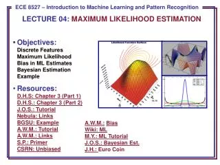
Example of ML Estimation • p(D|θ)is called the likelihood of θwith respect to the data. • The value of θthat maximizes this likelihood, denoted , • is the maximum likelihood estimate (ML) of θ. • Given several training points • Top: candidate source distributions are shown • Which distribution is the ML estimate? • Middle: an estimate of the likelihood of the data as a function of θ(the mean) • Bottom: log likelihood
General Mathematics • The ML estimate is found by solving this equation: • The solution to this equation can be a global maximum, a local maximum, or even an inflection point. • Under what conditions is it a global maximum?
A class of estimators – maximum a posteriori (MAP) – maximize where describes the prior probability of different parameter values. Maximum A Posteriori Estimation • An ML estimator is a MAP estimator for uniform priors. • A MAP estimator finds the peak, or mode, of a posterior density. • MAP estimators are not transformation invariant (if we perform a nonlinear transformation of the input data, the estimator is no longer optimum in the new space). This observation will be useful later in the course.
because: Gaussian Case: Unknown Mean • Consider the case where only the mean, θ= μ,is unknown: which implies:
Gaussian Case: Unknown Mean • Substituting into the expression for the total likelihood: • Rearranging terms: • Significance???
Gaussian Case: Unknown Mean and Variance • Let θ= [μ,σ2]. The log likelihood of a SINGLE point is: • The full likelihood leads to:
Gaussian Case: Unknown Mean and Variance • This leads to these equations: • In the multivariate case: • The true covariance is the expected value of the matrix ,which is a familiar result.
Convergence of the Mean • Does the maximum likelihood estimate of the variance converge to the true value of the variance? Let’s start with a few simple results we will need later. • Expected value of the ML estimate of the mean:
Variance of the ML Estimate of the Mean • The expected value of xixj,, E[xixj,], will be μ2for i≠ j and μ2 + σ2 otherwise since the two random variables are independent. • The expected value of xi2 will be μ2+ σ2. • Hence, in the summation above, we have n2-n terms with expected value μ2and n terms with expected value μ2+ σ2. • Thus, which implies: • We see that the variance of the estimate goes to zero as n goes to infinity, and our estimate converges to the true estimate (error goes to zero).
Variance Relationships • We will need one more result: Note that this implies: • Now we can combine these results. Recall our expression for the ML estimate of the variance:
Covariance Expansion • Expand the covariance and simplify: • One more intermediate term to derive:
Biased Variance Estimate • Substitute our previously derived expression for the second term:
Expectation Simplification • Therefore, the ML estimate is biased: However, the ML estimate converges (and is MSE). • An unbiased estimator is: • These are related by: which is asymptotically unbiased. See Burl, AJWills and AWM for excellent examples and explanations of the details of this derivation.
Summary • Discriminant functions for discrete features are completely analogous to the continuous case (end of Chapter 2). • To develop an optimal classifier, we need reliable estimates of the statistics of the features. • In Maximum Likelihood (ML) estimation, we treat the parameters as having unknown but fixed values. • Justified many well-known results for estimating parameters (e.g., computing the mean by summing the observations). • Biased and unbiased estimators. • Convergence of the mean and variance estimates.

